
What VLOOKUP Actually Does
VLOOKUP searches for a value in the first column of a table, then pulls back a value from another column in that same row. Think of it like looking up a name in a phone book: you find the name (the part you search), then read across to get the number (the part you retrieve).
It’s the function most Excel users learn first — and also the one that causes the most frustration, because it has quirks (like only being able to look right, never left) that aren’t obvious until they break your formula. This guide covers the syntax, four real examples, the exact errors you’ll hit and how to fix them, and when you should use XLOOKUP or INDEX-MATCH instead.
Syntax
| Argument | What it means |
|---|---|
| lookup_value | The value you’re searching for |
| table_array | The full range containing your data — the search column must be the first column in this range |
| col_index_num | Which column (counting from the left of table_array) to pull the result from — 1st column = 1, 2nd = 2, etc. |
| range_lookup | FALSE = exact match (use this 95% of the time). TRUE or omitted = approximate match |
VLOOKUP vs XLOOKUP vs INDEX-MATCH — Which Should You Use?
Here’s how VLOOKUP actually compares to XLOOKUP and INDEX-MATCH, so you can pick the right one.
| VLOOKUP | XLOOKUP | INDEX-MATCH | |
|---|---|---|---|
| Can look left of the search column? | ❌ No | ✅ Yes | ✅ Yes |
| Breaks if you insert a new column? | ✅ Yes (it will) | ❌ No | ❌ No |
| Available in older Excel versions? | ✅ Yes | ❌ 365/2021+ only | ✅ Yes |
| Easiest to learn? | ✅ Yes | ✅ Yes | ❌ Steeper curve |
| Handles errors gracefully? | Needs IFERROR wrapper | ✅ Built-in [if_not_found] | Needs IFERROR wrapper |
Bottom line: if you have Excel 365, use XLOOKUP going forward — it fixes VLOOKUP’s two biggest problems (can’t look left, breaks when columns are inserted). If you’re on an older Excel version or sharing files with people who are, VLOOKUP is still the safe, universal choice. INDEX-MATCH is worth learning once you’re comfortable, since it’s the most flexible of the three, but it’s not necessary for most day-to-day use.
When to Use VLOOKUP
Use it whenever you need to pull matching information from a table — looking up an employee’s salary from their ID, pulling a product price from a SKU, matching a student’s grade to their score, or cross-referencing data between two sheets.
What It Returns
The value found in your specified column, in the same row as the matching lookup_value. If no match is found, it returns #N/A.
Extra Notes Before You Start
- If range_lookup is FALSE and no exact match exists, you’ll get #N/A.
- For approximate matches (TRUE), the first column of your table must be sorted ascending, or you’ll get wrong results silently — this is the #1 cause of “VLOOKUP is giving me the wrong answer” complaints.
- col_index_num must be a positive whole number.
- VLOOKUP is case-insensitive — it treats “Apple” and “apple” as the same.
Examples of the Excel VLOOKUP Function
Here are a few examples of using the VLOOKUP function in Excel:
Example 1: Basic Lookup
You have an employee table and want to find a salary by employee ID.
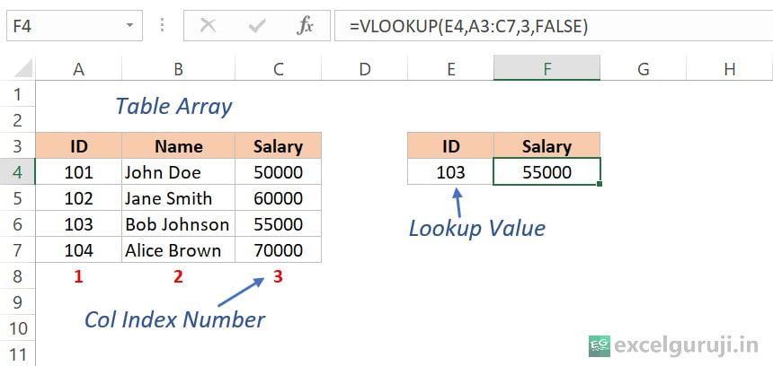
Formula: =VLOOKUP(E4,A3:C7,3,FALSE)
- E4 — the ID you’re searching for
- A3:C7 — your full data range
- 3 — salary is in the 3rd column of that range
- FALSE — exact match only
Result: looks up employee ID 103, finds it in column A, returns the value from column 3 (salary) — 55000.
Example 2: Approximate Match (Grading Scale)
A teacher wants to auto-assign letter grades based on test scores using a grade lookup table.
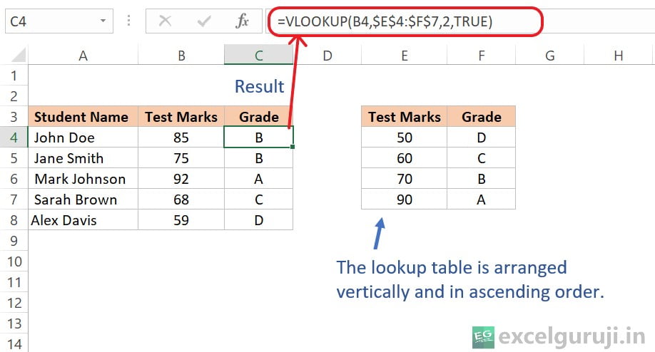
Formula: =VLOOKUP(B4,$E$4:$F$7,2,TRUE)
The TRUE here means VLOOKUP finds the closest value at or below the score — this only works correctly if your grade table is sorted from lowest to highest score.
Example 3: Exact Match (Survey Ratings)
A customer satisfaction survey rates service on a 1–4 scale, and you want to convert the number into a label like “Good” or “Excellent.”
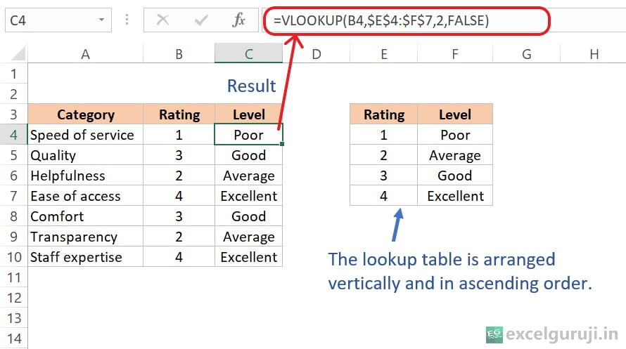
Formula: =VLOOKUP(B4,$E$4:$F$7,2,FALSE)
FALSE here matters — with rating data like this, an approximate match could silently return the wrong label if a rating doesn’t exist in your table.
Example 4: Two-Way Lookup (VLOOKUP + MATCH)
You’re managing monthly sales data across products, and need to look up a specific product’s sales for a specific month — a two-dimensional lookup.
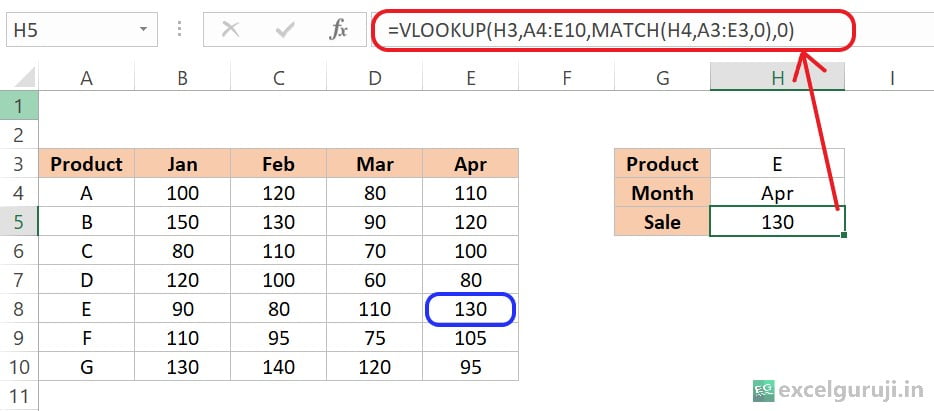
Formula: =VLOOKUP(H3,A4:E10,MATCH(H4,A3:E3,0),0)
Instead of hardcoding the column number, MATCH(H4,A3:E3,0) finds which column “Apr” sits in automatically. This means if you add or reorder month columns, the formula still works — a small trick that solves one of VLOOKUP’s biggest weaknesses.
Common VLOOKUP Errors (And How to Fix Them)
This is usually the part people are actually stuck on when they search — not the syntax, but why the formula isn’t working.
#N/A — “No match found”
Almost always one of: a typo in the lookup value, extra spaces in your data (use TRIM() to check), or the value genuinely doesn’t exist in the table. Wrap your formula in =IFERROR(VLOOKUP(…), “Not found”) to show a clean message instead of the error.
Wrong value returned (not an error, just incorrect)
Usually caused by using TRUE / omitting the last argument when you meant FALSE. Approximate match is the default if you leave it blank — this trips up more people than any other VLOOKUP mistake.
#REF! error
Your col_index_num is pointing to a column that doesn’t exist in your table_array — often happens after deleting a column. Double-check your range still has enough columns.
VLOOKUP works, then breaks after you insert a column
This is VLOOKUP’s biggest structural flaw — inserting a column shifts your data but not your hardcoded col_index_num. This is the single best reason to switch to XLOOKUP if you have access to it.
Formula returns 0 instead of blank
Happens when the matched cell is genuinely empty. Wrap it: =IF(VLOOKUP(…)=””,””,VLOOKUP(…)).
VLOOKUP Only Looks Right — Never Left
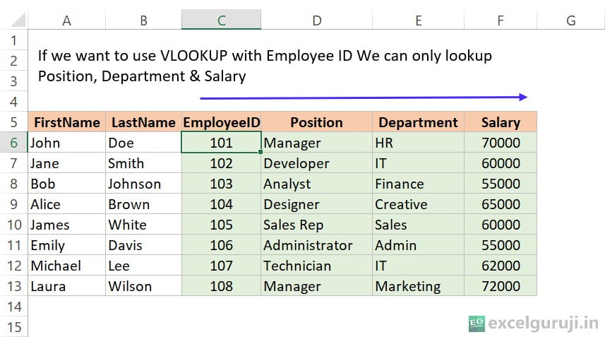
VLOOKUP’s search column must be the leftmost column of your range — it can only retrieve data from columns to the right of it. If you need to pull information from a column to the left of your lookup value, VLOOKUP simply can’t do it — you’ll need XLOOKUP or INDEX-MATCH instead.
Practice File
Download the file below and work through all four examples yourself:
Download Excel File For PracticeFrequently Asked Questions (FAQs)
Can VLOOKUP search in multiple columns?
No — it only searches the first column of your table_array.
Is VLOOKUP case-sensitive?
No, it treats uppercase and lowercase as identical.
What happens if no match is found?
It returns #N/A. Wrap the formula in IFERROR() to handle this gracefully.
Can VLOOKUP search a different worksheet or workbook?
Yes — reference the sheet name in your table_array, e.g. =VLOOKUP(A2,Sheet2!A:C,3,FALSE).
What happens with duplicate values in the first column?
VLOOKUP returns only the first match it finds, top to bottom — even if there are duplicates further down.
Should I switch to XLOOKUP?
If you’re on Excel 365 or 2021+, yes, for any new formulas — it’s more flexible and doesn’t break when columns are inserted. Keep VLOOKUP knowledge for files shared with people on older Excel versions.
Related Excel Functions