Mastering Excel LOOKUP Function: A Comprehensive Guide to Searching and Retrieving Data in Excel (With Practice File)

Excel LOOKUP Function
Excel-LOOKUP-Function

When to Use the Excel LOOKUP Function in Excel

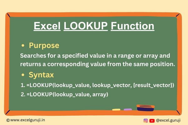
The LOOKUP function in Excel is a versatile tool used to search for a value in a range and return a corresponding value from the same position in another range. It is particularly handy when dealing with large datasets or when you need to quickly find specific information based on certain criteria.

What Excel LOOKUP Function Returns

The Excel LOOKUP function returns a value either from a one-row or one-column range or from an array. The function searches for the lookup_value in the first row or column of the specified range and returns the corresponding value from the same position in the last row or column of that range.

Syntax of Excel LOOKUP Function

The Excel LOOKUP function has two variations in syntax, and each serves a specific purpose:

Syntax 1:

=LOOKUP(lookup_value, lookup_vector, [result_vector])

This syntax is used when you want to find a value in a one-row or one-column range (lookup_vector) and return the corresponding value from another one-row or one-column range (result_vector). If result_vector is omitted, the function returns the corresponding value from lookup_vector.

Syntax 2:

=LOOKUP(lookup_value, array)

This syntax is employed when you want to find a value in an array and return the corresponding value from the same position in that array.

Input Arguments

Here are the input arguments for both variations of the Excel LOOKUP function:

lookup_value: The value you want to search for in the lookup_vector or array.

lookup_vector: For Syntax 1, this is the range that contains the values you want to compare with the lookup_value. It can be a one-row or one-column range or an array.

result_vector: (Optional) For Syntax 1, this is the range that contains the values to be returned. If omitted, the function returns the corresponding value from the lookup_vector.

array: For Syntax 2, this is the array in which you want to find the lookup_value.

Extra Notes

● The lookup_vector must be in ascending order. If it is not, the LOOKUP function may return #N/A/ error.

● If the lookup_value is smaller than the smallest value in the lookup_vector, the LOOKUP function returns the #N/A error.

● If the lookup_value is larger than the largest value in the lookup_vector, the LOOKUP function matches the largest value that is less than or equal to lookup_value.

● LOOKUP is not case-sensitive

Examples of the Excel LOOKUP Function

Here are few examples of using the LOOKUP function in Excel:

Example 1: Basic Usage

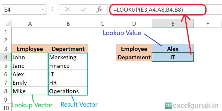
Imagine you are managing a small team, and you have a list of employees along with their respective departments. You receive a request to find the department for a specific employee. To accomplish this task, you decide to use the LOOKUP function in Excel.
Excel-LOOKUP-Function-Example-1

Here is an explanation of the formula: =LOOKUP(E3,A4:A8,B4:B8)

  • E3 contains the lookup value, which is “Alex” in this case.
  • A4:A8 is the range where Excel will search for the lookup value. In this example, it is the range of employee names (John, Jane, Alex, Emily, Mike).
  • B4:B8 is the range from which Excel will return the corresponding value. In this case, it is the range of departments (Marketing, Finance, IT, HR, Operations).

So, the formula is essentially saying, “Look for the value in cell E3 (‘Alex’) in the range A4:A8 (employee names), and return the corresponding value from the range B4:B8 (departments).

Example 2: Using an Array for Lookup

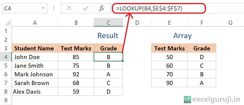
Imagine you are a teacher managing a class of students, and you have recently conducted a test. Each student’s test marks need to be graded. You have a list of students along with their respective test marks, and you want to use a lookup table to determine the corresponding grades. So, let us see in the following example how to use the LOOKUP function.
Excel LOOKUP Function Example 2

Here is an explanation of the formula: =LOOKUP(B4,$E$4:$F$7)

  • B4 contains the test marks for a specific student, let’s say, Alex Davis, which is 59 in this case.
  • $E$4:$F$7 represents the array table where Excel will look for the corresponding grade based on the test marks. The $ symbols before the column and row references make the range absolute, meaning it won’t change when you copy the formula to other cells.

So, the formula is saying, “Look for the value in cell B4 (test marks for Alex Davis) in the range of test marks in the array table (E4:E7), and return the corresponding grade from the second column of the array table (F4:F7).

Practice with Real Examples: Download the Attached Excel File

To facilitate your hands-on practice, I have attached an Excel file. You can download the file and work through the few examples I shared earlier, applying the LOOKUP function in Excel.

Download Excel File For Practice

If you have any questions or need assistance, feel free to reach out. Enjoy practicing and mastering the Excel LOOKUP function!

Conclusion

In conclusion, the Excel LOOKUP function, with its two syntax variations, is an essential tool for quickly searching and retrieving information from a dataset. Whether you are working with product lists, employee data, or any other dataset, the LOOKUP function can streamline your tasks and make your Excel experience more efficient.

As with any Excel function, practice is key to mastering the LOOKUP function. Experiment with different scenarios and datasets to enhance your proficiency. Start using the LOOKUP function today and take your Excel skills to the next level!

Frequently Asked Questions (FAQs)

Q1: Can the LOOKUP function be used to search for values in multiple columns?

A1: Yes, the LOOKUP function can search for values in both one-row and one-column ranges, making it versatile for various data structures.

Q2: Is the Excel LOOKUP function case-sensitive?

A2: No, the Excel LOOKUP function is not case-sensitive.

Q3: What happens if the lookup_value is not found in the lookup_vector or array?

A3: In such cases, the LOOKUP function returns the #N/A error. You can use the IFERROR function to handle this situation and display a custom message.

Q4: Can the result_vector be in a different worksheet?

A4: Yes, the result_vector can be in a different worksheet. Simply reference the range using the appropriate worksheet notation.

Q5: Are there alternatives to the LOOKUP function for searching values in Excel?

A5: Yes, alternatives include functions like VLOOKUP, HLOOKUP, and INDEX-MATCH, each with its own advantages and use cases.

Other Related Excel Functions

Mastering Excel VLOOKUP Function: A Comprehensive Guide to Enhance Your Data Analysis Skills

Unlocking Data Mastery with Excel HLOOKUP Function: A Comprehensive Guide for Efficient Horizontal Data Lookup

Mastering Excel FILTER Function: A Comprehensive Guide for Data Filtering

Master Data Selection with Excel TAKE Function

Excel DROP Function: A Comprehensive Guide to Unlocking Excel’s Potential:

Join me on Instagram, YouTube and WhatApp Channel for your daily dose of valuable tips and tricks! Catch insightful videos that will enhance your knowledge and skills. Don’t miss out – follow me now!

VLOOKUP in Excel: The Complete Guide (With Real Examples, Errors, and When to Use XLOOKUP Instead)

Excel VLOOKUP function guide - lookup value in a table using VLOOKUP formula

What VLOOKUP Actually Does

VLOOKUP searches for a value in the first column of a table, then pulls back a value from another column in that same row. Think of it like looking up a name in a phone book: you find the name (the part you search), then read across to get the number (the part you retrieve).

It’s the function most Excel users learn first — and also the one that causes the most frustration, because it has quirks (like only being able to look right, never left) that aren’t obvious until they break your formula. This guide covers the syntax, four real examples, the exact errors you’ll hit and how to fix them, and when you should use XLOOKUP or INDEX-MATCH instead.

Syntax

=VLOOKUP(lookup_value, table_array, col_index_num, [range_lookup])
ArgumentWhat it means
lookup_valueThe value you’re searching for
table_arrayThe full range containing your data — the search column must be the first column in this range
col_index_numWhich column (counting from the left of table_array) to pull the result from — 1st column = 1, 2nd = 2, etc.
range_lookupFALSE = exact match (use this 95% of the time). TRUE or omitted = approximate match

VLOOKUP vs XLOOKUP vs INDEX-MATCH — Which Should You Use?

Here’s how VLOOKUP actually compares to XLOOKUP and INDEX-MATCH, so you can pick the right one.

 VLOOKUPXLOOKUPINDEX-MATCH
Can look left of the search column?❌ No✅ Yes✅ Yes
Breaks if you insert a new column?✅ Yes (it will)❌ No❌ No
Available in older Excel versions?✅ Yes❌ 365/2021+ only✅ Yes
Easiest to learn?✅ Yes✅ Yes❌ Steeper curve
Handles errors gracefully?Needs IFERROR wrapper✅ Built-in [if_not_found]Needs IFERROR wrapper

Bottom line: if you have Excel 365, use XLOOKUP going forward — it fixes VLOOKUP’s two biggest problems (can’t look left, breaks when columns are inserted). If you’re on an older Excel version or sharing files with people who are, VLOOKUP is still the safe, universal choice. INDEX-MATCH is worth learning once you’re comfortable, since it’s the most flexible of the three, but it’s not necessary for most day-to-day use.

When to Use VLOOKUP

Use it whenever you need to pull matching information from a table — looking up an employee’s salary from their ID, pulling a product price from a SKU, matching a student’s grade to their score, or cross-referencing data between two sheets.

What It Returns

The value found in your specified column, in the same row as the matching lookup_value. If no match is found, it returns #N/A.

Extra Notes Before You Start

  • If range_lookup is FALSE and no exact match exists, you’ll get #N/A.
  • For approximate matches (TRUE), the first column of your table must be sorted ascending, or you’ll get wrong results silently — this is the #1 cause of “VLOOKUP is giving me the wrong answer” complaints.
  • col_index_num must be a positive whole number.
  • VLOOKUP is case-insensitive — it treats “Apple” and “apple” as the same.

Examples of the Excel VLOOKUP Function

Here are a few examples of using the VLOOKUP function in Excel:

Example 1: Basic Lookup

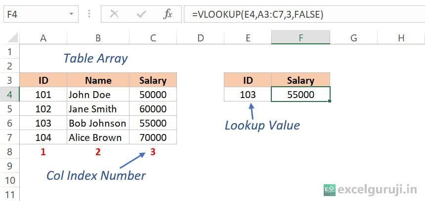
You have an employee table and want to find a salary by employee ID.

Excel VLOOKUP Function Example 1

Formula: =VLOOKUP(E4,A3:C7,3,FALSE)

    • E4 — the ID you’re searching for
    • A3:C7 — your full data range
    • 3 — salary is in the 3rd column of that range
    • FALSE — exact match only

    Result: looks up employee ID 103, finds it in column A, returns the value from column 3 (salary) — 55000.

    Example 2: Approximate Match (Grading Scale)

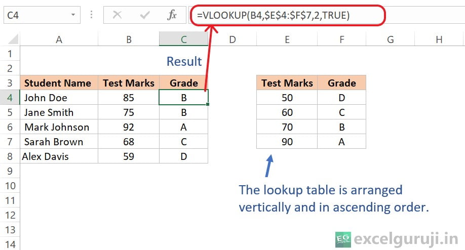
    A teacher wants to auto-assign letter grades based on test scores using a grade lookup table.

    Excel VLOOKUP Function Example 2

    Formula: =VLOOKUP(B4,$E$4:$F$7,2,TRUE)

    The TRUE here means VLOOKUP finds the closest value at or below the score — this only works correctly if your grade table is sorted from lowest to highest score.

    Example 3: Exact Match (Survey Ratings)

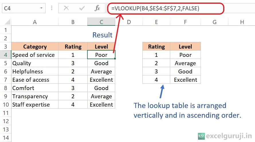
    A customer satisfaction survey rates service on a 1–4 scale, and you want to convert the number into a label like “Good” or “Excellent.”

    Excel-VLOOKUP-Function-Example-3

    Formula: =VLOOKUP(B4,$E$4:$F$7,2,FALSE)

    FALSE here matters — with rating data like this, an approximate match could silently return the wrong label if a rating doesn’t exist in your table.

    Example 4: Two-Way Lookup (VLOOKUP + MATCH)

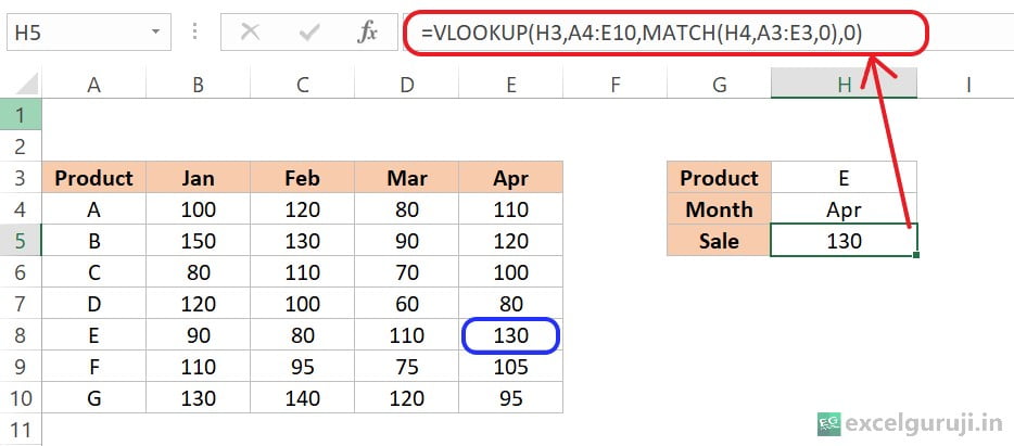
    You’re managing monthly sales data across products, and need to look up a specific product’s sales for a specific month — a two-dimensional lookup.

    Excel-VLOOKUP-Function-Example-5

    Formula: =VLOOKUP(H3,A4:E10,MATCH(H4,A3:E3,0),0)

    Instead of hardcoding the column number, MATCH(H4,A3:E3,0) finds which column “Apr” sits in automatically. This means if you add or reorder month columns, the formula still works — a small trick that solves one of VLOOKUP’s biggest weaknesses.

    Common VLOOKUP Errors (And How to Fix Them)

    This is usually the part people are actually stuck on when they search — not the syntax, but why the formula isn’t working.

    #N/A“No match found”
    Almost always one of: a typo in the lookup value, extra spaces in your data (use TRIM() to check), or the value genuinely doesn’t exist in the table. Wrap your formula in =IFERROR(VLOOKUP(…), “Not found”) to show a clean message instead of the error.

    Wrong value returned (not an error, just incorrect)
    Usually caused by using TRUE / omitting the last argument when you meant FALSE. Approximate match is the default if you leave it blank — this trips up more people than any other VLOOKUP mistake.

    #REF! error
    Your col_index_num is pointing to a column that doesn’t exist in your table_array — often happens after deleting a column. Double-check your range still has enough columns.

    VLOOKUP works, then breaks after you insert a column
    This is VLOOKUP’s biggest structural flaw — inserting a column shifts your data but not your hardcoded col_index_num. This is the single best reason to switch to XLOOKUP if you have access to it.

    Formula returns 0 instead of blank
    Happens when the matched cell is genuinely empty. Wrap it: =IF(VLOOKUP(…)=””,””,VLOOKUP(…)).

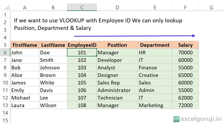
    VLOOKUP Only Looks Right — Never Left

    VLOOKUP’s search column must be the leftmost column of your range — it can only retrieve data from columns to the right of it. If you need to pull information from a column to the left of your lookup value, VLOOKUP simply can’t do it — you’ll need XLOOKUP or INDEX-MATCH instead.

    Excel-VLOOKUP-Function-Example-4-1

    Practice File

    Download the file below and work through all four examples yourself:

    Download Excel File For Practice

    Frequently Asked Questions (FAQs)

    Can VLOOKUP search in multiple columns?

    No — it only searches the first column of your table_array.

    Is VLOOKUP case-sensitive?

    No, it treats uppercase and lowercase as identical.

    What happens if no match is found?

    It returns #N/A. Wrap the formula in IFERROR() to handle this gracefully.

    Can VLOOKUP search a different worksheet or workbook?

    Yes — reference the sheet name in your table_array, e.g. =VLOOKUP(A2,Sheet2!A:C,3,FALSE).

    What happens with duplicate values in the first column?

    VLOOKUP returns only the first match it finds, top to bottom — even if there are duplicates further down.

    Should I switch to XLOOKUP?

    If you’re on Excel 365 or 2021+, yes, for any new formulas — it’s more flexible and doesn’t break when columns are inserted. Keep VLOOKUP knowledge for files shared with people on older Excel versions.

    Related Excel Functions

    Unlocking Data Mastery with Excel HLOOKUP Function: A Comprehensive Guide for Efficient Horizontal Data Lookup

    Excel HLOOKUP Function

    Excel-HLOOKUP-Function

    When to Use the Excel HLOOKUP Function in Excel

    The HLOOKUP function in Excel is a powerful tool when you need to search for a value in the first row of a range and retrieve a corresponding value in the same column from a specified row. This function is particularly useful when dealing with large datasets, tables, or spreadsheets with headers and data organized horizontally.

    What Excel HLOOKUP Function Returns

    The Excel HLOOKUP function returns a value by searching for a specified lookup value in the first row of a table or range and then retrieving the corresponding value from a specified row. It essentially performs a horizontal lookup in a table.

    Syntax of Excel HLOOKUP Function

    The syntax of the Excel HLOOKUP function is as follows

    =HLOOKUP(lookup_value, table_array, row_index_num, [range_lookup])

    Input Arguments

    Here are the input arguments for the Excel HLOOKUP function:

    lookup_value: The value to search for in the first row of the table.

    table_array: The range of cells that contains the data. The first row of this range should contain the values to be searched.

    row_index_num: The row number in the table from which to retrieve the value.

    range_lookup [optional]: A logical value that specifies whether to find an exact match or an approximate match. If TRUE or omitted, it searches for an approximate match. If FALSE, it searches for an exact match.

    Extra Notes

    ● If no match is found, the function returns #N/A.

    ● The table_array must be arranged in a way that the first row contains the values to be searched, and the subsequent rows contain the corresponding data.

    ● The row_index_num must be a positive integer.

    ● If range_lookup is TRUE or omitted, the values in the first row of table_array must be sorted in ascending order.

    ● Excel HLOOKUP function is case-insensitive, treating uppercase and lowercase characters as the same.

    Examples of the Excel HLOOKUP Function

    Here are few examples of using the HLOOKUP function in Excel

    Example 1: Basic Usage

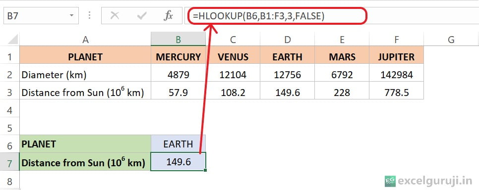
    Imagine you are an astronomer working with a dataset that contains information about various planets, including their diameters and distances from the Sun1. Your goal is to use the HLOOKUP function in Excel to quickly retrieve specific details about a particular planet based on input.

    Excel-HLOOKUP-Function-Example-1

    Here is an explanation of the formula: =HLOOKUP(B6, B1:F3, 3, FALSE)

    • B6: This is the lookup value. In this case, you are looking for the value in cell B6, which is likely a planet name (e.g., “EARTH”).
    • B1:F3: This is the table array. It represents the range of cells that contains the data. In this context, it is likely the dataset with information about planets, their diameters, and distances from the Sun.
    • 3: This is the row index number. It indicates from which row in the table array the function should retrieve the corresponding value. In this case, you specified 3, so it will look in the third row of the table array.
    • FALSE: This is the range_lookup parameter. When set to FALSE, it indicates that an exact match is required. In other words, the function will look for the exact value specified in B6 in the first row of the table array.

    Example 2: Approximate Match With HLOOKUP

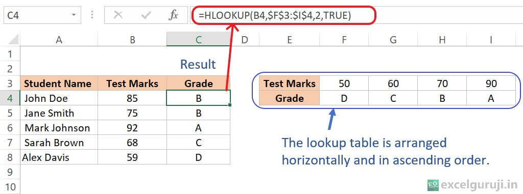
    Suppose you are a teacher managing a class of students, and you want to automatically assign grades based on their test marks. You have a list of students with their respective test marks, and you have established a grading scale with specific grade ranges. To streamline the grading process, you decide to use a lookup array to automatically determine the grade for each student.

    Excel-HLOOKUP-Function-Example-2

    Here is an explanation of the formula: =HLOOKUP(B4,$F$3:$I$4,2,TRUE)

    • B4 is the cell containing the test marks for a specific student.
    • $F$3:$I$4 is the lookup array, where the dollar signs ($) make the reference absolute.
    • 2 is the row index number, indicating that the function should return the corresponding grade from the second row of the lookup array.
    • TRUE means it will perform an approximate match, finding the closest (lesser) value in the first row of the lookup array.

    Example 3: Exact Match With HLOOKUP

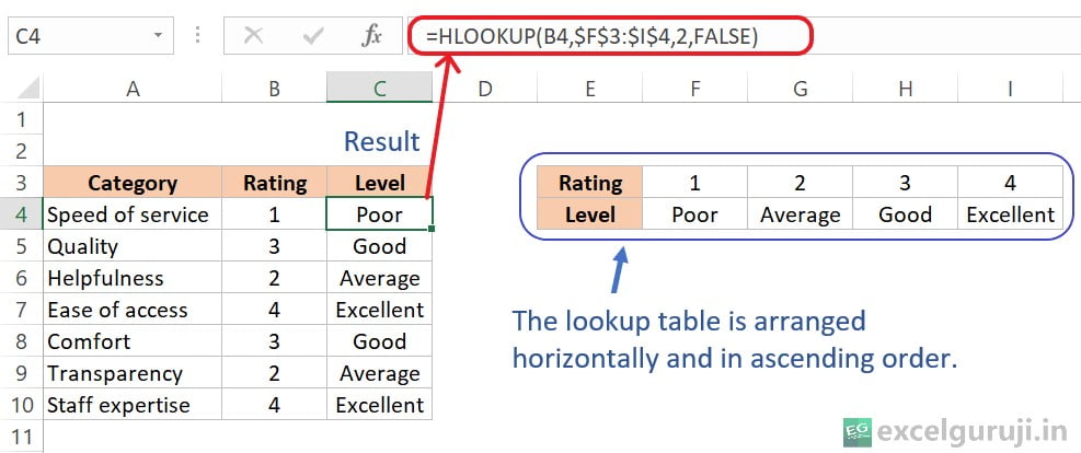
    Imagine you work for a company that provides services to customers, and you have conducted a customer satisfaction survey to gather feedback on various aspects of your service. You asked customers to rate different service attributes on a scale from 1 to 4, where 1 is “Poor”, 2 is “Average”, 3 is “Good” and 4 is “Excellent”. The survey covered categories like speed of service, quality, helpfulness, ease of access, comfort, transparency, and staff expertise.

    Excel-HLOOKUP-Function-Example-3

    Here is an explanation of the formula: =HLOOKUP(B4, $F$3:$I$4, 2, FALSE)

    • B4: This is the cell reference containing the “Rating” in data table.
    • $F$3:$I$4: This is the lookup array or table. It is a where the first row contains the ratings (1, 2, 3, 4), and the second row contains the corresponding levels (Poor, Average, Good, Excellent). The $ symbols before the column and row references make the range absolute, meaning it won’t change when you copy the formula to other cells.
    • 2: This parameter indicates that the function should return the value from the second row of the lookup table (which contains the levels).
    • FALSE: This is the range_lookup parameter, and setting it to FALSE means that the function should find an exact match for the rating. If an exact match is not found, it returns an error (#N/A).

    Practice with Real Examples: Download the Attached Excel File

    To facilitate your hands-on practice, I have attached an Excel file. You can download the file and work through the three examples I shared earlier, applying the HLOOKUP function in Excel.

    Download Excel File

    If you have any questions or need assistance, feel free to reach out. Enjoy practicing and mastering the Excel HLOOKUP function!

    Conclusion

    In conclusion, the Excel HLOOKUP function is a valuable tool for searching and retrieving data from horizontally organized tables. Whether you are working with sales data, project timelines, or any dataset where information is arranged horizontally, the Excel HLOOKUP function can streamline your data retrieval tasks.

    As with any Excel function, practice is key to mastering the HLOOKUP function. Experiment with different scenarios and datasets to enhance your proficiency. Start incorporating the HLOOKUP function into your Excel repertoire today and take your data analysis skills to the next level!

    Frequently Asked Questions (FAQs)

    Q1: Can the Excel HLOOKUP function be used to search for values in the first column of a table?

    A1: No, the Excel HLOOKUP function is designed exclusively for searching in the first row of a table.

    Q2: Is the HLOOKUP function case-sensitive?

    A2: No, the HLOOKUP function is not case-sensitive.

    Q3: What happens if no match is found using HLOOKUP?

    A3: If no match is found, the function returns #N/A.

    Q4: Can the row_index_num be a negative number?

    A4: No, the row_index_num must be a positive integer.

    Q5: How does the HLOOKUP function handle duplicates in the first row of the table?

    A5: The HLOOKUP function returns the first matching value found in the first row of the table, even if there are duplicates.

    Other Related Excel Functions

    Mastering Excel VLOOKUP Function: A Comprehensive Guide to Enhance Your Data Analysis Skills

    Mastering Excel FILTER Function: A Comprehensive Guide for Data Filtering

    Master Data Selection with Excel TAKE Function

    Excel DROP Function: A Comprehensive Guide to Unlocking Excel’s Potential:

    Join me on Instagram, YouTube and WhatApp Channel for your daily dose of valuable tips and tricks! Catch insightful videos that will enhance your knowledge and skills. Don’t miss out – follow me now!
    1. Nasa.gov ↩︎

    Mastering Excel COUNTIFS Function for Advanced Data Analysis (With Video Tutorial)

    Excel COUNTIFS Function

    Excel COUNTIFS Function

    When to Use the Excel COUNTIFS Function in Excel

    The COUNTIFS function in Excel is an incredibly useful tool when you need to count cells based on multiple criteria. It allows you to specify conditions that data must meet to be included in the count, making it ideal for complex data analysis and reporting.

    What Excel COUNTIFS Function Returns

    The Excel COUNTIFS function returns the count of cells that meet multiple criteria. It helps you find the number of cells that satisfy all the conditions you specify.

    Syntax of Excel COUNTIFS Function

    The syntax of the Excel COUNTIFS function is as follows:

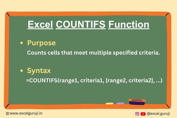
    =COUNTIFS(range1, criteria1, [range2, criteria2], …)

    Input Arguments

    Here are the input arguments for the Excel COUNTIFS function:

    range1: The first range of cells that you want to apply the first criteria to.

    criteria1: The condition that must be met in the first range.

    [range2, criteria2]: Additional pairs of range and criteria that you can include to add more conditions.

    Extra Notes

    ● The COUNTIFS function is not case-sensitive. It treats uppercase and lowercase letters as identical.

    ● Cells are counted only if all the specified conditions are satisfied.

    ● You can use up to 127 pairs of criteria and criteria ranges.

    ● Criteria can make use of wildcard characters like “?,” “*”, and “~” to enhance flexibility in your data analysis.

    ● If the criteria contain text, it should be enclosed in double quotation marks (” “).

    ● Criteria do not require cell references to be enclosed in quotes, for example, “>=”& A1.

    ● You can use logical operators (>, <, =, etc.) in your criteria for more advanced filtering.

    Examples of the Excel COUNTIFS Function

    Here are a few examples to illustrate how to use the COUNTIFS function in Excel:

    Example 1: Counting Products with Specific Criteria

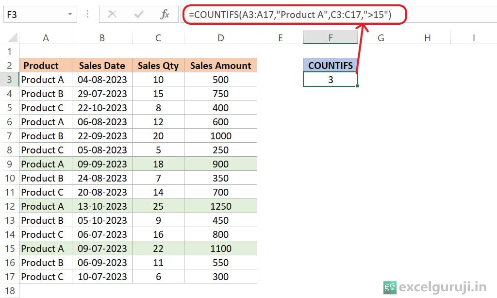
    Imagine you have a product list with columns for Product names (in column A), Sales Date (in column B), Sales Qty (in column C), and Sales Amount (in column D). Your goal is to count the occurrences of “Product A” with sales quantities exceeding “15”. Use the following formula:

    Excel-COUNTIFS-Function-Example-1

    This formula counts the number of products that meet both criteria.

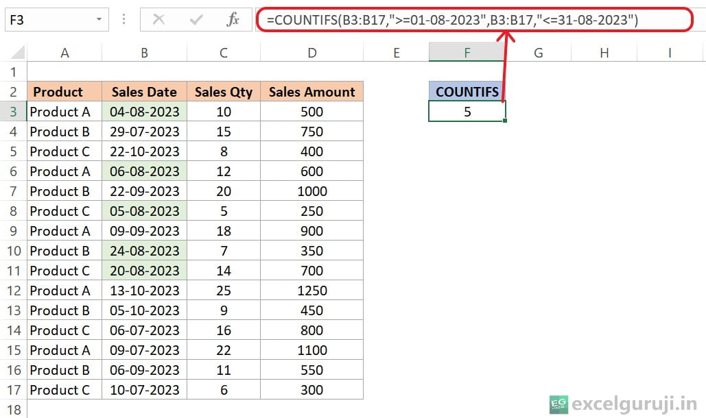
    Example 2: Counting Sales in a Specific Month

    Suppose you want to count how many sales were made in the specific month. Use the following formula:

    Excel-COUNTIFS-Function-Example-2

    This formula will count the number of sales entries corresponding to August 2023.

    Understanding Wildcards in Excel

    In Excel, wildcards are special characters or character combinations employed as placeholders in functions, formulas, and search operations. They enhance the flexibility and power of searches, comparisons, and filtering. The primary wildcards in Excel are the asterisk (*) and the question mark (?).

    The asterisk (*) signifies any number of characters, even none. For instance, when searching for “*apple”, it matches words like “apple”, “Custard apple”, serving as a placeholder for multiple characters.

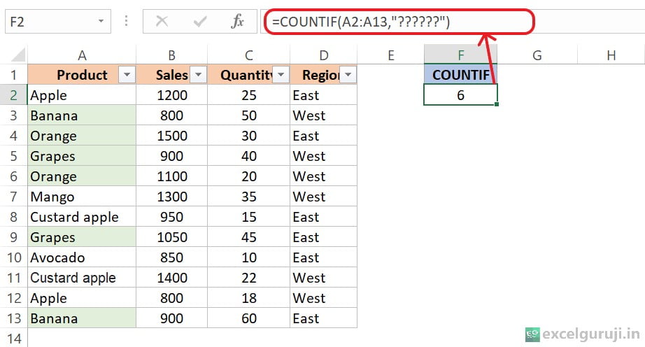
    The question mark (?) represents a single character. For example, searching for “??????” matches strings that contain 6 characters. Which you can see in the image below.

    Excel COUNTIF Function Example 4

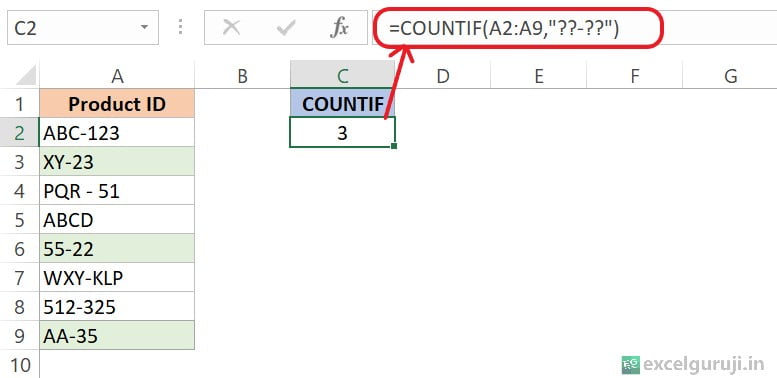
    searching for “??-??” specifies that you are looking for cells with a specific pattern. In this case, “??-??” means two question marks followed by a hyphen (-) and then followed by two more question marks.

    Excel COUNTIF Function Example 5

    Wildcards are especially valuable when dealing with data that varies in spelling, format, or content. They simplify the process of finding, manipulating, and analyzing data in Excel spreadsheets.

    Excel COUNTIFS Function – Video Tutorial

    Excel Countifs Function – Video Tutorial

    Practice Workbook

    Download Free Excel File For Practice

    Conclusion

    In conclusion, the Excel COUNTIFS function is an essential tool for counting cells that meet multiple criteria. Whether you are working with sales data, product lists, or any other type of data, the Excel COUNTIFS function simplifies the process of obtaining precise counts based on complex conditions.

    Remember that Excel offers a wide range of functions to help you manipulate and analyze data. As with any function, practice is key to mastering it.

    Experiment with different scenarios and datasets to get a better grasp of how Excel COUNTIFS function can be applied effectively in your projects.

    Frequently Asked Questions (FAQs)

    Q1: Can I use the Excel COUNTIFS function to count cells based on both text and numerical criteria?

    A1: Yes, the Excel COUNTIFS function is versatile and allows you to use a combination of text, numerical, and date criteria.

    Q2: Can I count cells that meet multiple criteria in different columns?

    A2: Absolutely. You can use Excel COUNTIFS to count cells based on conditions in multiple columns by specifying additional [range2, criteria2] pairs in the function.

    Q3: What if I want to count cells that meet any of the specified criteria, not all?

    A3: In that case, you should use the Excel COUNTIF function, which counts cells based on a single condition. The Excel COUNTIFS function is specifically for counting cells that meet all the specified conditions.

    Q4: Is it possible to count cells based on a range of dates, for example, all orders placed within a specific month?

    A4: Yes, you can count cells based on date ranges by specifying appropriate date criteria in the Excel COUNTIFS function. For instance, you can count all orders within a specific month by using criteria like “>=” the start of the month and “<=” the end of the month.

    Q5: Can I use Excel COUNTIFS to count cells that meet conditions in non-contiguous ranges?

    A5: Unfortunately, Excel COUNTIFS function doesn’t support counting cells based on non-contiguous ranges. You may need to use other functions or techniques in such cases.

    Other Related Excel Functions

    Unlocking the Power of Excel COUNT Function for Accurate Numeric Data Analysis

    Mastering Excel COUNTA Function: Counting Non-Empty Cells Made Easy

    Excel COUNTBLANK Function: How to Count Empty Cells in Excel

    Join me on Instagram, YouTube and WhatApp Channel for your daily dose of valuable tips and tricks! Catch insightful videos that will enhance your knowledge and skills. Don’t miss out – follow me now!
    Mastering the Excel COUNTIF Function for Efficient Data Analysis (With Video Tutorial)

    Excel COUNTIF Function

    Excel-COUNTIF-Function

    When to Use the Excel COUNTIF Function in Excel

    The COUNTIF function in Excel is used when you need to tally the occurrences of a particular condition or criterion within a given range of cells.

    It is a versatile function that can be applied in various situations, such as tracking sales, monitoring progress, or identifying outliers in your data.

    What Excel COUNTIF Function Returns

    The Excel COUNTIF function returns the count of cells that meet the specified condition. The condition is defined by you and can be based on text, numbers, dates, or other criteria. It provides a simple way to quantify the data that matches your criteria.

    Syntax of Excel COUNTIF Function

    The syntax of the Excel COUNTIF function is as follows:

    =COUNTIF(range, criteria)

    Input Arguments

    Here are the input arguments for the Excel COUNTIF function:

    range: The range of cells you want to count values in. This can be a range reference, a named range, or an array.

    criteria: The criteria that determine which cells to count. This can be a specific value, expression, or text that Excel uses to evaluate the cells in the specified range.

    Extra Notes

    ● The COUNTIF function is not case-sensitive. It treats uppercase and lowercase letters as identical.

    ● You can use wildcards in the criteria to match patterns or partial values within the cells.

    ● If the criteria contain text, it should be enclosed in double quotation marks (” “).

    ● Criteria do not require cell references to be enclosed in quotes, for example, “>=”& A1.

    ● You can use logical operators (>, <, =, etc.) in your criteria for more advanced filtering.

    ● When referring to another workbook that is not open, COUNTIF will result in a #VALUE error.

    Examples of the Excel COUNTIF Function

    Here are few examples of using the COUNTIF function in Excel:

    Example 1: Basic Usage

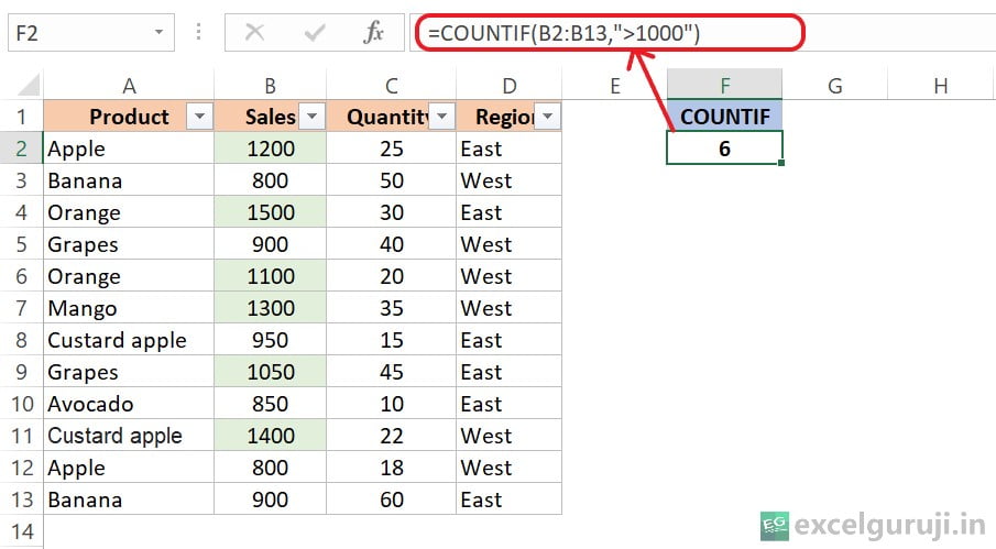
    Suppose you have a list of sales figures in column B, and you want to count how many sales are greater than 1000. You can use the following formula:

    Excel COUNTIF Function Example 1

    Example 2: Using a Cell Reference for Criteria

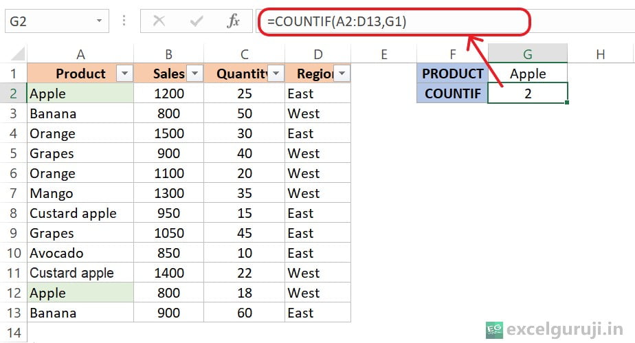
    If you have a specific criterion in a cell, you can reference it in your formula. For instance, if cell G1 contains the criteria “Apple” and you want to count how many times “Apple” appears in a range from A2 to A13, you can use:

    Excel COUNTIF Function Example 2

    Utilizing cell references in formulas offers flexibility, simplifies maintenance, and decreases the chances of errors, enhancing the efficiency and user-friendliness of your spreadsheet.

    When you input a cell reference and subsequently alter the value in that cell, your formula will adjust automatically to show the updated value. This enables dynamic, real-time adjustments without requiring direct formula modifications.

    Example 3: Using Wildcards

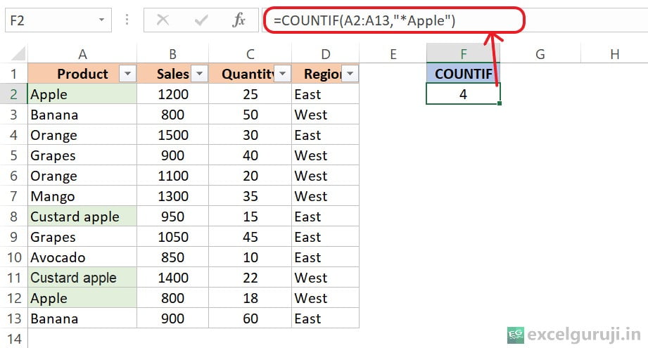
    Suppose you have a list of products in column A, and you want to count how many products contain the word “apple” anywhere in their names. You can use a wildcard (*) like this:

    Excel COUNTIF Function Example 3
    Understanding Wildcards in Excel

    In Excel, wildcards are special characters or character combinations employed as placeholders in functions, formulas, and search operations. They enhance the flexibility and power of searches, comparisons, and filtering. The primary wildcards in Excel are the asterisk (*) and the question mark (?).

    The asterisk (*) signifies any number of characters, even none. For instance, when searching for “*apple”, it matches words like “apple”, “Custard apple”, serving as a placeholder for multiple characters.

    The question mark (?) represents a single character. For example, searching for “??????” matches strings that contain 6 characters. Which you can see in the image below.

    Excel COUNTIF Function Example 4

    searching for “??-??” specifies that you are looking for cells with a specific pattern. In this case, “??-??” means two question marks followed by a hyphen (-) and then followed by two more question marks.

    Excel COUNTIF Function Example 5

    Wildcards are especially valuable when dealing with data that varies in spelling, format, or content. They simplify the process of finding, manipulating, and analyzing data in Excel spreadsheets.

    Example 4: Counting World Cup Wins with Excel COUNTIF

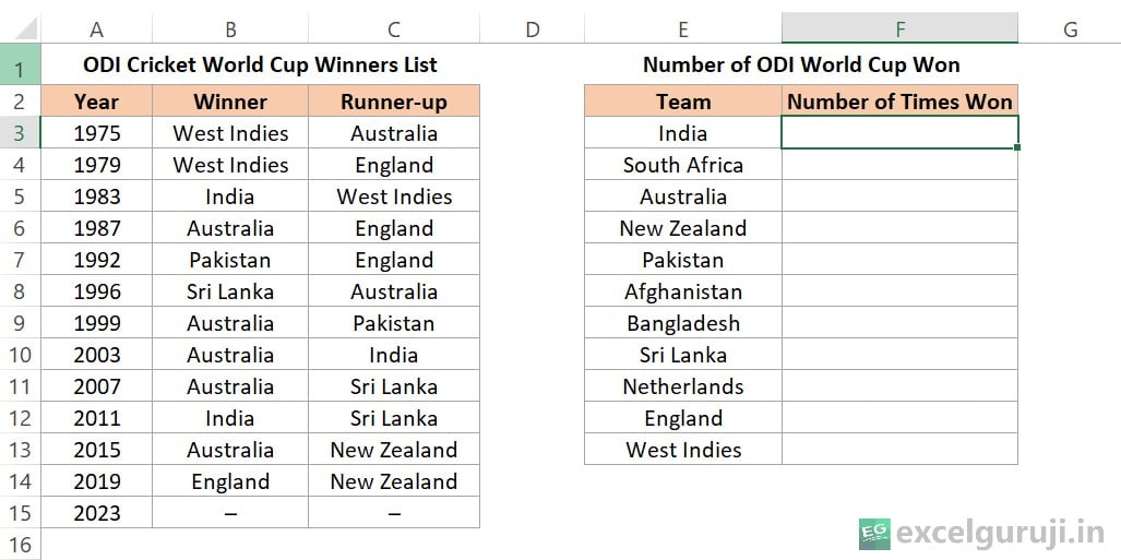
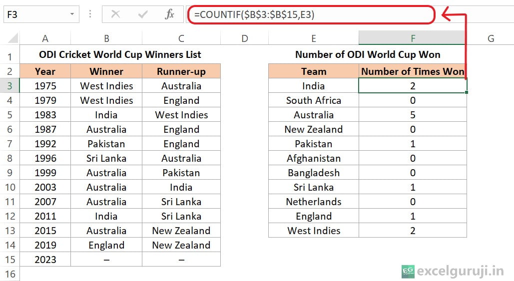
    In this example, we will use the Excel COUNTIF function to analyze historical data on the winners of the ODI Cricket World Cup1. We want to determine how many times a specific team has won the World Cup over the years.

    Excel-COUNTIF-Function-Example-6-1

    Now, let’s say we want to count how many times a particular team has won the ODI Cricket World Cup. To do this, we will use the COUNTIF function. In column F, we will input the following formula:

    Excel-COUNTIF-Function-Example-7

    Here is what each part of the formula does: =COUNTIF($B$3:$B$15, E3)

    • COUNTIF is the Excel function we are using to count cells that meet a specific condition.
    • $B$3:$B$15 represents absolute references (Press F4 to lock references) to the range of cells containing the winners of the ODI Cricket World Cup.
    • E3 contains the team name we want to count, which is “India” in this case.

    The formula counts the number of times “India” appears in the Winner column (column B), which corresponds to the number of times India has won the World Cup. In this example, it returns a value of “2”, indicating that India has won the ODI Cricket World Cup two times.

    Excel COUNTIF Function – Video Tutorial

    Excel Countif Function – Video Tutorial

    Practice Workbook

    Download Free Excel File For Practice

    Conclusion

    In conclusion, the Excel COUNTIF function is an essential tool for counting cells that meet specific criteria. It empowers you to make data-driven decisions, analyze information, and gain insights from your Excel spreadsheets.

    Whether you are dealing with numbers, text, or dates, the COUNTIF function simplifies the process of data analysis.

    Remember that Excel is a versatile tool, and mastering its functions can significantly enhance your productivity and proficiency. Start using the COUNTIF function today, and unlock new possibilities in your data management and analysis tasks!

    Frequently Asked Questions (FAQs)

    Q1: Can the Excel COUNTIF function be used to count cells that meet multiple criteria?

    A1: Yes, you can count cells that meet multiple criteria by using multiple Excel COUNTIF functions and combining their results using logical operators like “+” or “*”.

    Q2: Is the Excel COUNTIF function case-sensitive?

    A2: No, the Excel COUNTIF function is not case-sensitive; it treats uppercase and lowercase letters as identical.

    Q3: Can the Excel COUNTIF function count cells based on a partial match or pattern?

    A3: Yes, you can use wildcards in the criteria to match patterns or partial values within the cells.

    Q4: Can I use logical operators in the criteria for the Excel COUNTIF function?

    A4: Yes, you can use logical operators like “>”, “<“, “=”, etc.

    Q5: What is the difference between COUNTIF and COUNTIFS functions in Excel?

    A5: COUNTIF is used to count cells based on a single criterion, whereas COUNTIFS allows you to count cells based on multiple criteria simultaneously.

    Other Related Excel Functions

    Unlocking the Power of Excel COUNT Function for Accurate Numeric Data Analysis

    Mastering Excel COUNTA Function: Counting Non-Empty Cells Made Easy

    Excel COUNTBLANK Function: How to Count Empty Cells in Excel

    Join me on Instagram, YouTube and WhatApp Channel for your daily dose of valuable tips and tricks! Catch insightful videos that will enhance your knowledge and skills. Don’t miss out – follow me now!
    1. ODI Cricket World Cup Winners List from 1975 to 2023, Updated ↩︎

    Excel COUNTBLANK Function: How to Count Empty Cells in Excel (With Video Tutorial)

    Excel COUNTBLANK Function

    Excel-COUNTBLANK-Function

    When to Use the Excel COUNTBLANK Function in Excel

    The COUNTBLANK function1 in Excel is a handy tool when you need to count the number of empty or blank cells within a specified range. It can be particularly useful in data analysis, auditing spreadsheets, or assessing the completeness of data.

    What Excel COUNTBLANK Function Returns

    The Excel COUNTBLANK function returns the count of cells within a given range that are empty or contain no data.

    Syntax of Excel COUNTBLANK Function

    The syntax of the Excel COUNTBLANK function is as follows:

    =COUNTBLANK(range)

    Input Arguments

    Here is the input argument for the Excel COUNTBLANK function:

    range: This is the range of cells that you want to count the blank cells within. It can be a reference to a cell range, a named range, or a combination of cells.

    Extra Notes

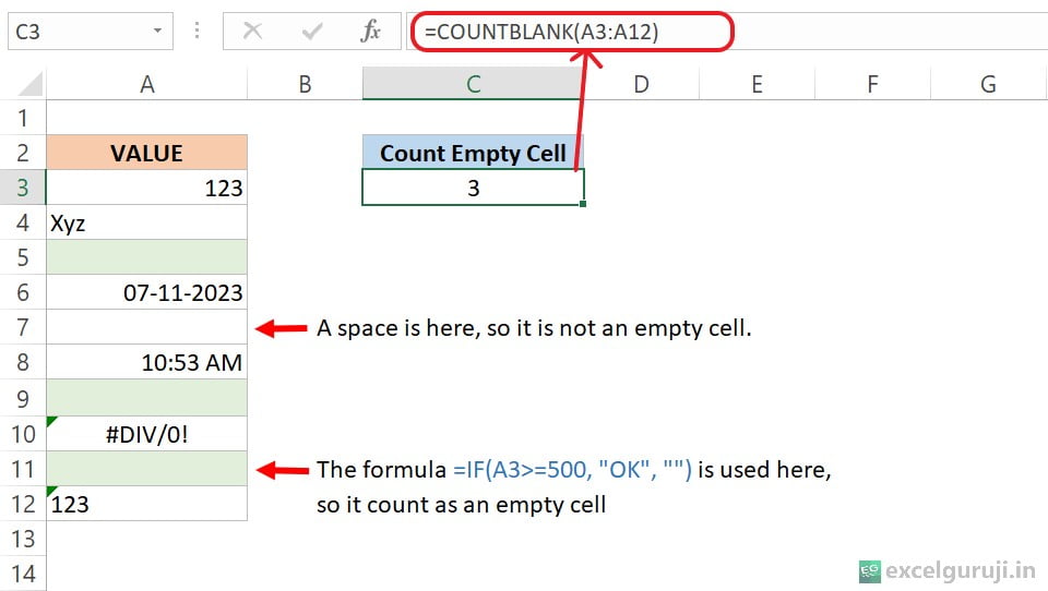
    ● The COUNTBLANK function considers cells with no data, including those with empty text, as blank cells.

    ● If a cell contains a formula that returns an empty result (“”), it is also counted as a blank cell.

    ● Cells with space characters or non-printable characters are not considered blank, they need to be empty.

    Examples of the Excel COUNTBLANK Function

    Here are a few examples of using the COUNTBLANK function in Excel:

    Excel-COUNTBLANK-Function-Example

    Unseen Influences: COUNTBLANK and Invisible Characters

    Invisible characters refer to characters or symbols that are present in a text but are not typically visible when you look at the text.

    These characters can be things you can’t see, like spaces or special codes. Sometimes, these hidden things can change how the text looks or acts, but you might not notice them at first.

    When using functions like COUNTBLANK in Excel, it is crucial to be aware of the presence of invisible characters, as they can impact the results, as demonstrated in the image above.

    To avoid the situation where invisible characters can impact your results when using functions like COUNTBLANK in Excel, you can use the “Go To Special” option in Excel to identify and deal with cells containing specific types of content, including blank cells. Here is how you can do it:

    • Select the desired range.
    • Open the Go To dialog (use Ctrl + G).
    • Click on “Special”.
    • Choose “Blanks”

    This feature is helpful when you want to identify and work with empty cells, which might be hiding invisible characters or unexpected data. It allows you to clean up your data and ensure its integrity for functions like COUNTBLANK in Excel.

    Excel COUNTBLANK Function – Video Tutorial

    Excel Countblank Function – Video Tutorial

    Practice Workbook

    Download Free Excel File For Practice

    Conclusion

    In conclusion, the Excel COUNTBLANK function is a valuable tool for assessing the completeness of your data by counting the number of empty or blank cells within a given range.

    Whether you are working with large datasets or auditing spreadsheets, the COUNTBLANK function can save you time and help ensure data quality.

    Remember that Excel offers a wide range of functions to manipulate and analyze data, and mastering them takes practice.

    Don’t hesitate to experiment and explore different applications of the COUNTBLANK function in your own projects. Start using the COUNTBLANK function today and enhance your Excel skills.

    Frequently Asked Questions (FAQs)

    Q1: Can the COUNTBLANK function count cells with spaces or non-printable characters as blank cells?

    A1: No, the COUNTBLANK function counts only cells that are truly empty or contain no data.

    Q2: How can I count non-blank cells within a range?

    A2: To count non-blank cells within a range, you can use the COUNTA function, which counts cells that contain data, including text, numbers, and formulas.

    Other Related Excel Functions

    Unlocking the Power of Excel COUNT Function for Accurate Numeric Data Analysis

    Join me on Instagram, YouTube and WhatApp Channel for your daily dose of valuable tips and tricks! Catch insightful videos that will enhance your knowledge and skills. Don’t miss out – follow me now!
    1. Excel COUNTBLANK Function ↩︎

    Mastering Excel COUNTA Function: Counting Non-Empty Cells Made Easy (With Video Tutorial)

    Excel COUNTA Function

    Excel-COUNTA-Function

    When to Use the Excel COUNTA Function in Excel

    The COUNTA function in Excel comes in handy in several scenarios, including:

    Data Validation: You can use COUNTA to ensure that a specific number of cells in a range are filled with data before proceeding with calculations or processes.

    Data Analysis: When working with datasets, you may want to know how many entries are complete or contain information, and COUNTA helps you do just that.

    Error Checking: COUNTA is useful for spotting missing or incomplete data, which can be critical for maintaining data accuracy and integrity.

    What Excel COUNTA Function Returns

    The Excel COUNTA function returns the count of non-empty cells within a specified range. It does not just count numbers, it considers any data type, including text, dates, errors, logical values, and more.

    Syntax of Excel COUNTA Function

    The syntax of the Excel COUNTA function is as follows:

    =COUNTA(value1, [value2], …)

    Input Arguments

    Here are the input arguments for the Excel COUNTA function:

    value1, value2, …: These are the values or ranges you want to count. You can provide up to 255 arguments.

    Extra Notes

    Empty Cells: COUNTA does not count empty cells, which are cells with no data, formula results, or errors.

    Mixed Data Types: COUNTA treats all data types (text, numbers, logical values, errors) equally, so it counts them all.

    Blanks in Formulas: Cells with formulas that return blank are counted as non-empty.

    Examples of the Excel COUNTA Function

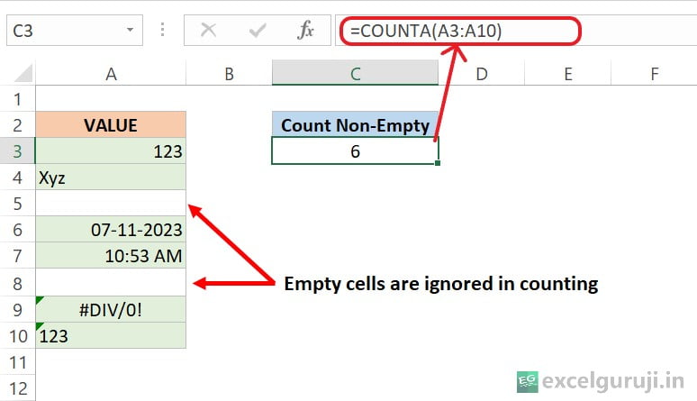
    To count non-empty cell in a range, use the following formula:

    Excel-COUNTA-Function-Example

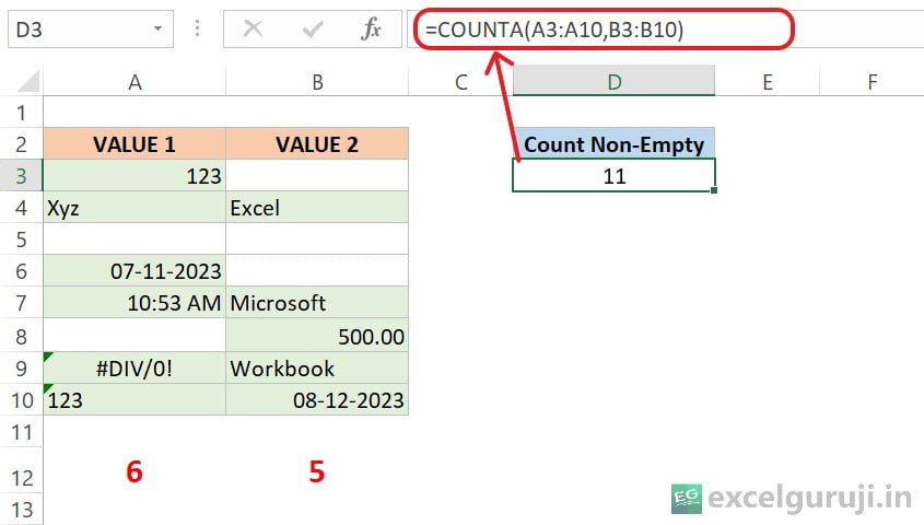
    To count non-empty cell in multiple ranges, use the following formula:

    Excel COUNTA Function Example 2

    Unseen Influences: COUNTA and Invisible Characters

    Invisible characters refer to characters or symbols that are present in a text but are not typically visible when you look at the text.

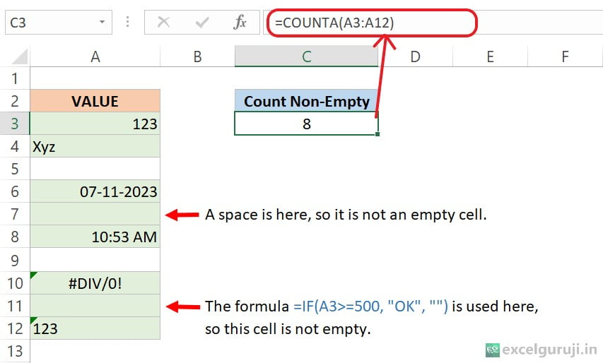
    These characters can include non-printing characters, such as spaces, tabs, line breaks, characters that match the background color, and other formatting or control characters. In some cases, these characters can impact the formatting and behavior of the text, yet they may not be immediately apparent to the reader.

    When using functions like COUNTA in Excel, it is crucial to be aware of the presence of invisible characters, as they can impact the results, as demonstrated in the image below.

    Excel-COUNTA-Function-Example-3

    To avoid the situation where invisible characters can impact your results when using functions like COUNTA in Excel, you can use the “Go To Special” option in Excel to identify and deal with cells containing specific types of content, including blank cells. Here is how you can do it:

    • Select the desired range.
    • Open the Go To dialog (use Ctrl + G).
    • Click on “Special”.
    • Choose “Blanks”

    This feature is helpful when you want to identify and work with empty cells, which might be hiding invisible characters or unexpected data. It allows you to clean up your data and ensure its integrity for functions like COUNTA in Excel.

    Excel COUNTA Function – Video Tutorial

    Excel Counta Function – Video Tutorial

    Practice Workbook

    Download Free Excel File For Practice

    Conclusion

    In conclusion, the Excel COUNTA function is an essential tool for counting non-empty cells in Excel. Whether you are managing data, validating information, or analyzing datasets, COUNTA simplifies the process of ensuring data completeness and accuracy.

    Excel is a powerful tool, and understanding functions like COUNTA can greatly enhance your productivity and decision-making. So, start using the COUNTA function in your spreadsheets today and take your Excel skills to new heights!

    Frequently Asked Questions (FAQs)

    Q1: Can the COUNTA function count empty cells?

    A1: No, the COUNTA function only counts non-empty cells, disregarding empty cells.

    Q2: Does the Excel COUNTA function differentiate between data types (text, numbers, errors, etc.)?

    A2: No, the Excel COUNTA function counts all data types as long as the cell is not empty.

    Q3: What if I want to count only numeric values in a range?

    A3: If you want to count only numeric values, you can use the COUNT function, which counts cells containing numbers.

    Q4: Can the Excel COUNTA function count cells with formulas that return a blank value?

    A4: Yes, the Excel COUNTA function counts cells with formulas that return blank values as non-empty.

    Q5: What function should I use if I want to count empty cells specifically?

    A5: To count empty cells, you can use the COUNTBLANK function.

    Other Related Excel Functions

    Join me on Instagram, YouTube and WhatApp Channel for your daily dose of valuable tips and tricks! Catch insightful videos that will enhance your knowledge and skills. Don’t miss out – follow me now!
    Unlocking the Power of Excel COUNT Function for Accurate Numeric Data Analysis (With Video Tutorial)

    Excel COUNT Function

    Excel-COUNT-Function

    When to Use the Excel COUNT Function in Excel

    The COUNT function in Excel is a powerful tool that allows you to count the number of cells containing numbers within a given range. It is particularly useful in data analysis, statistics, and when you need to keep track of numerical values in your spreadsheets.

    What Excel COUNT Function Returns

    The Excel COUNT function returns the count of numeric values within a specified range.

    Syntax of Excel COUNT Function

    The syntax of the Excel COUNT function is as follows:

    =COUNT(value1, [value2], …)

    Input Arguments

    Here are the input arguments for the Excel COUNT function:

    value1, value2, …: These are the values or cell references you want to count. You can provide up to 255 arguments, and the function will count the numeric values within this list.

    Extra Notes

    ● The COUNT function ignores empty cells, text, and logical values (TRUE/FALSE).

    ● Error values and text that cannot be interpreted as numbers are excluded from the count.

    Examples of the Excel COUNT Function

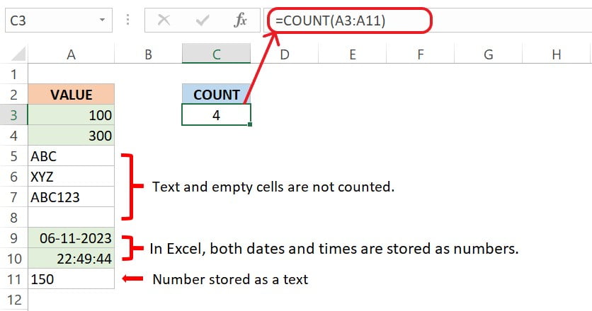
    To count numeric values in a range, use the following formula:

    Excel-COUNT-Function-Example-1

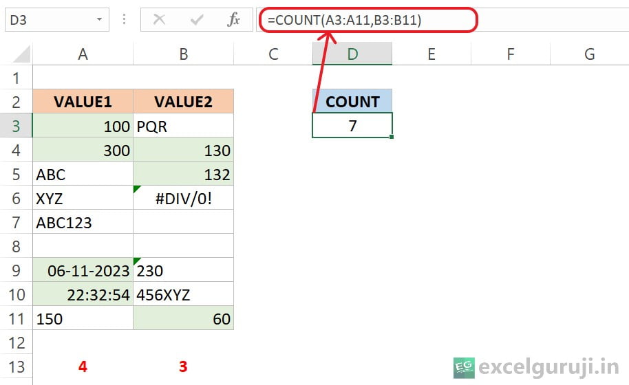
    To count numeric values in multiple ranges, use the following formula:

    Excel COUNT Function Example 2

    Excel COUNT Function – Video Tutorial

    Excel Count Function – Video Tutorial

    Practice Workbook

    Download Free Excel File For Practice

    Conclusion

    In conclusion, the Excel COUNT function is a valuable tool for counting numeric values within a range. Whether you are working on financial data, statistics, or any other numeric data analysis, the COUNT function can help you quickly gather the information you need.

    Remember, Excel offers a wide range of functions that can streamline your tasks and improve your efficiency. Practice and explore different applications of the COUNT function in your own projects to enhance your Excel skills.

    Frequently Asked Questions (FAQs)

    Q1: Can the COUNT function count non-numeric values?

    A1: No, the COUNT function only counts numeric values. Non-numeric values, empty cells, and text are ignored.

    Q2: Does the COUNT function differentiate between different data types?

    A2: No, the COUNT function treats all numeric values equally, regardless of their data type.

    Q3: Can I use the COUNT function with multiple ranges?

    A3: Yes, you can provide multiple ranges or values as arguments to the COUNT function, and it will count the numeric values across all the specified ranges.

    Q4: Is there a similar function to count non-numeric values in Excel?

    A4: Yes, you can use the COUNTA function to count all values, including non-numeric ones, within a range.

    Other Related Excel Functions

    Excel COUNTBLANK Function: How to Count Empty Cells in Excel

    Join me on Instagram, YouTube and WhatApp Channel for your daily dose of valuable tips and tricks! Catch insightful videos that will enhance your knowledge and skills. Don’t miss out – follow me now!
    Mastering Excel FILTER Function: A Comprehensive Guide for Data Filtering

    Excel FILTER Function

    Excel FILTER Function

    When to Use the Excel FILTER Function in Excel

    The FILTER function in Excel is a powerful tool for filter specific data from a range based on specified criteria.

    It is incredibly handy for managing and analyzing large datasets, helping you quickly retrieve the information you need while leaving out the rest.

    What Excel FILTER Function Returns

    The Excel FILTER function returns a dynamic array that includes only the rows from a given range that meet the specified conditions. This function is particularly useful when you want to filter data based on one or multiple criteria.

    Syntax of Excel FILTER Function

    The syntax of the Excel FILTER function is as follows:

    =FILTER(array, include, [if_empty])

    Input Arguments

    Here are the input arguments for the Excel FILTER function:

    array: This is the range of data that you want to filter. It can be a reference to a range of cells, a table, or an array.

    include: This is the array or range of cells where you specify the conditions that the data must meet to be included in the filtered results.

    [if_empty]: This argument is optional. You can use it to specify what should be returned if there are no matching results. If omitted, it will return #CALC! error.
    Extra Notes

    ● Excel FILTER function is exclusively accessible in Microsoft 365’s Excel and Excel for the web. To learn more about how to use Excel for Web for free. Watch 👇 this video

    How to Get Microsoft Excel for Free | Free Microsoft Office | Microsoft Office 365

    ● Make sure the include argument matches the size of the list, or FILTER will not work.

    ● You can also use multiple criteria to filter the data by providing an array of conditions.

    Examples of the Excel FILTER Function

    Here are few examples of using the FILTER function in Excel:

    Example 1: Basic Usage

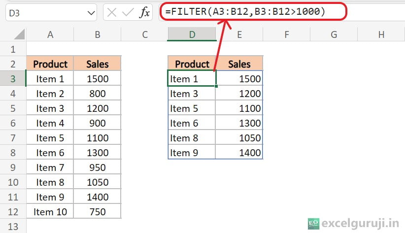
    Suppose you have a table of sales data in columns A and B. You want to filter the data to show only the rows where the sales value is greater than 1,000. In a new range, enter the following formula:

    Excel-FILTER-Function-Example-1-1

    Here is an explanation of the formula: =FILTER(A3:B12, B3:B12 > 1000)

    • A3:B12: This is the dataset or range of data you want to filter. In this example, it includes two columns: Product in column A and Sales in column B. The range starts from cell A3 and ends at B12.
    • B3:B12 > 1000: This part defines the condition for filtering. It specifies that only rows where the value in column B (Sales) is greater than 1000 should be included in the result.

    So, when you enter this formula, it will return a filtered list of rows from the original dataset (A3:B12), where the Sales value in column B is greater than 1000.

    Example 2: Using Multiple Criteria

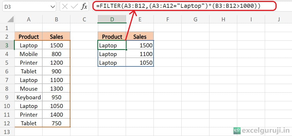
    Let’s say you have a list of products in column A, their sales in column B, and you want to filter the products that meet two criteria: the product should be a Laptop, and its sales should be more than 1000. In a new range, enter the following formula:

    Excel-FILTER-Function-Example-2

    =FILTER(A3:B12,(A3:A12=”Laptop”)*(B3:B12>1000))

    • A3:A12=”Laptop” : It selects rows where the corresponding cell in column A (Product) is equal to Laptop.
    • B3:B12>1000: It also checks if the corresponding cell in column B (Sales) is greater than 1000.

    In other words, it filters the data to show products that are labeled as Laptop and have sales exceeding 1000.

    Example 3: Handling Empty Results

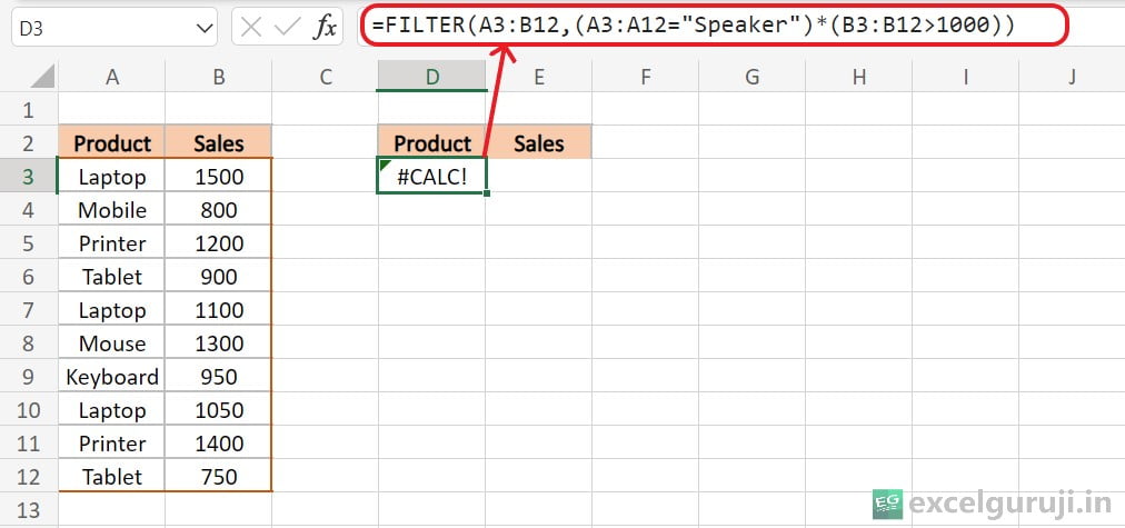
    If there are no matching results, the FILTER function will return an error by default. As shown in the formula below, when it doesn’t find a product named “Speaker” anywhere in the range from A3:A12, it gives a #CALC! error because it couldn’t find a matching result.

    Excel-FILTER-Function-Example-3

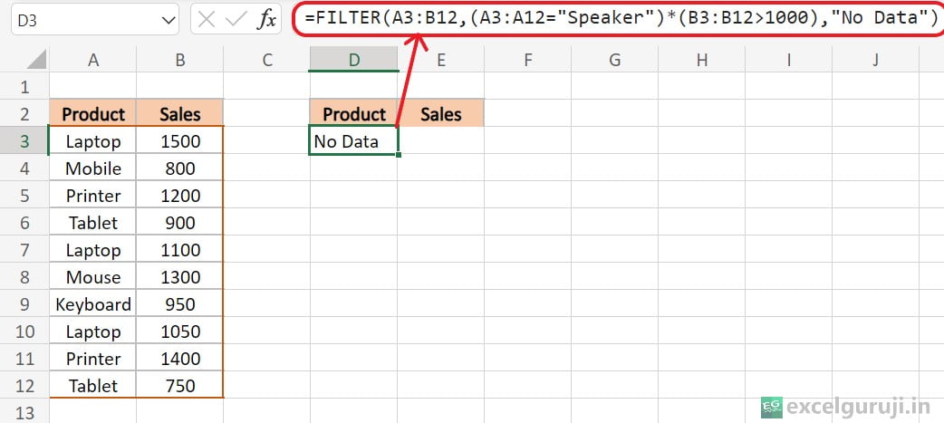
    In such cases, you can customize the error using an [if_empty] argument, as demonstrated in the following formula.

    Excel-FILTER-Function-Example-4

    Example 4: Dynamic Filtering with Cell References

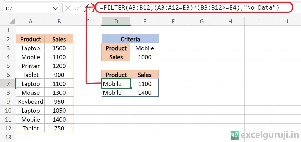
    Using cell references in formulas provides flexibility, ease of maintenance, and reduces the risk of errors, making your spreadsheet more efficient and user-friendly. If you enter a cell reference and later change the value in that cell, your formula will automatically update to reflect the new value.

    This allows for dynamic and real-time adjustments without the need to modify the formula itself.

    Excel FILTER Function Example 5

    In the image, you can observe how this formula dynamically updates its results as we change the values in cells E3 and E4. This level of flexibility allows for real-time adjustments without the need to alter the formula manually.

    Let’s Practice What You have Learned.

    Now, it is your turn to try out the Excel FILTER function. You can use the Excel file we have provided to practice and see how it works with sample data.

    If you have any questions or if you discover something interesting, please feel free to share your thoughts in the comments. Enjoy learning through hands-on experience!

    Conclusion

    In conclusion, the Excel FILTER function is a versatile tool that simplifies the process of extracting specific data from a large dataset.

    Whether you are working with sales records, inventory information, or any other dataset, the FILTER function can save you time and help you make more informed decisions.

    Like any Excel function, mastering FILTER takes practice. Don’t hesitate to experiment with different filtering criteria and explore its various applications in your own projects.

    Start using the FILTER function today and take your Excel skills to the next level!

    Frequently Asked Questions (FAQs)

    Q1: Can the FILTER function be used to filter data based on multiple conditions?

    A1: Yes, the Excel FILTER function is capable of filtering data based on single or multiple conditions. You can specify multiple criteria in the include argument.

    Q2: What happens if there are no matching results when using the FILTER function?

    A2: If there are no matching results, the FILTER function will return an error by default. You can use the [if_empty] argument to customize the output in such cases.

    Q3: Can the FILTER function return results in multiple cells?

    A3: Yes, the FILTER function can return results in multiple cells if there are multiple matching rows in the filtered data.

    Q4: Is the FILTER function case-sensitive?

    A4: No, the FILTER function is not case-sensitive by default. It treats text in a case-insensitive manner, so “Laptop” and “LAPTOP” would be considered the same when filtering with the FILTER function.

    Q5: What other Excel functions complement the FILTER function for data analysis?

    A5: Excel functions like SORT, SUMIFS, COUNTIFS, and AVERAGEIFS can be used in conjunction with the FILTER function to perform advanced data analysis and reporting.

    Other Related Excel Functions

    Excel CHOOSE Function: A Guide to Efficient Data Selection

    Mastering Excel CHOOSECOLS Function: Custom Data Extraction and Analysis

    Join me on Instagram, YouTube and WhatApp Channel for your daily dose of valuable tips and tricks! Catch insightful videos that will enhance your knowledge and skills. Don’t miss out – follow

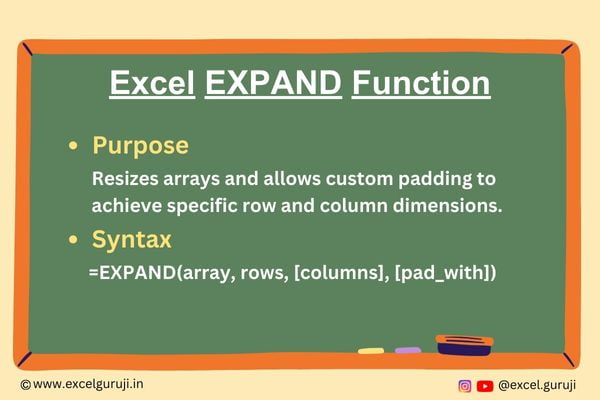
    Mastering Excel EXPAND Function: Resizing and Padding Arrays with Precision

    Excel EXPAND Function

    Excel EXPAND Function

    When to Use the Excel EXPAND Function in Excel

    The EXPAND function in Excel is essential when you want to modify the dimensions of an array to meet your data presentation needs.

    It is particularly useful in scenarios where you need to match the dimensions of one array with another, fill empty elements, or ensure consistent formatting for your data.

    What Excel EXPAND Function Returns

    The Excel EXPAND function returns an expanded or padded array based on your specified row and column dimensions. You can also choose what value to pad empty elements with, providing flexibility in managing your data arrays.

    Syntax of Excel EXPAND Function

    The syntax of the Excel EXPAND function is as follows:

    =EXPAND(array, rows, [columns], [pad_with])

    Input Arguments

    Here are the input arguments for the Excel EXPAND function:

    array: This is the array you want to expand or pad. It can be a range of cells, a reference to an array, or a direct array entry enclosed in curly braces.

    rows: The number of rows in the expanded array. If this argument is omitted or left empty, the number of rows in the result will match the original array.

    columns: The number of columns in the expanded array. If this argument is omitted or left empty, the number of columns in the result will match the original array.

    pad_with: The value with which to pad empty elements in the array. The default value is #N/A, but you can specify a different value if needed.

    Extra Notes

    ● Excel EXPAND function is exclusively accessible in Microsoft 365’s Excel and Excel for the web. To learn more about how to use Excel for Web for free. Watch 👇 this video

    How to Get Microsoft Excel for Free | Free Microsoft Office | Microsoft Office 365

    ● You are required to provide at least one argument, either the row argument or the column argument.

    ● When the number of specified rows is smaller than the row count in the array, the EXPAND function will yield a #VALUE! error.

    ● Likewise, if the number of specified columns is less than the column count in the array, the EXPAND function will also produce a #VALUE! error.

    Examples of the Excel EXPAND Function

    Let’s explore a few practical examples of the EXPAND function in Excel:

    Example 1: Enlarge the Array to a Specific Number of Rows

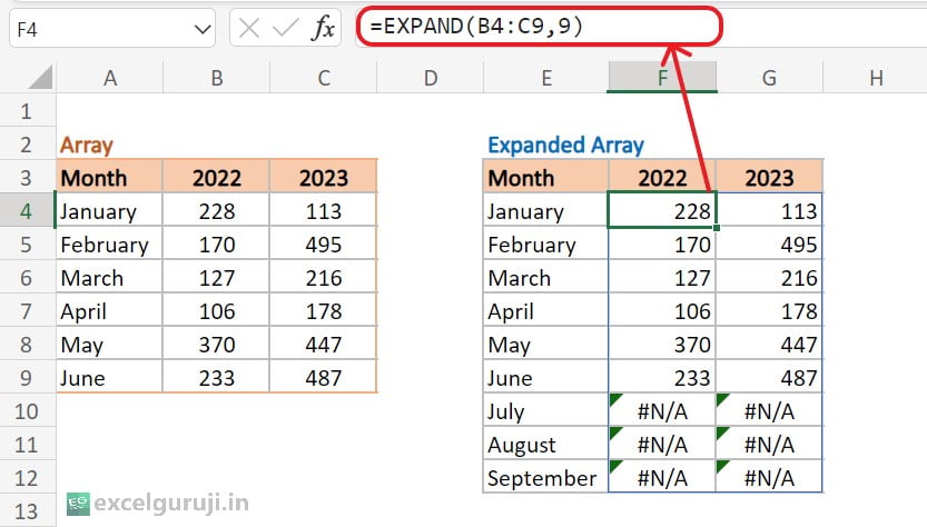
    Suppose you have a dataset, and you want to expand the array down to specific rows. You can do this using the following formula:

    Excel EXPAND Function Example 1

    The formula =EXPAND(B4:C9, 9) expands the array represented by the range B4:C9 to have a total of 9 rows. Let’s break it down step by step:

    • B4:C9 : This is the range in your Excel worksheet, which contains data or an array of values.
    • 9: The number of rows you want the array to have after expansion. In this case, it is asking to expand the array to a total of 9 rows.

    So, when you enter this formula, it takes the original array within the range B4:C9 and adds enough rows to make the array have a total of 9 rows.

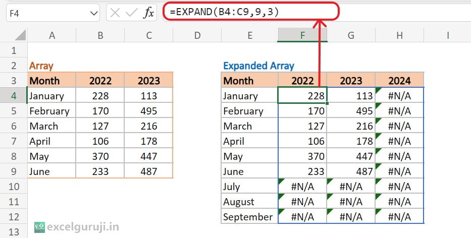
    Example 2: Enlarge the Array to a Specific Number of Rows and Columns

    Suppose you have a dataset, and you want to expand the array to specific rows and column. You can do this using the following formula:

    Excel EXPAND Function Example 2

    =EXPAND(B4:C9,9,3)

    • B4:C9 : This is the range in your Excel worksheet, which contains data or an array of values.
    • 9: The number of rows you want the array to have after expansion. In this case, it is asking to expand the array to a total of 9 rows.
    • 3: The number of columns you want the array to have after expansion. In this case, it is asking to expand the array to a total of 3 columns.

    So, when you enter this formula, it takes the original array within the range B4:C9 and expands it to have 9 rows and 3 columns.

    Example 3: Enlarge the Array With Padding

    Suppose you have a dataset, and you want to expand the array to specific rows and columns with a padding value. You can do this using the following formula:

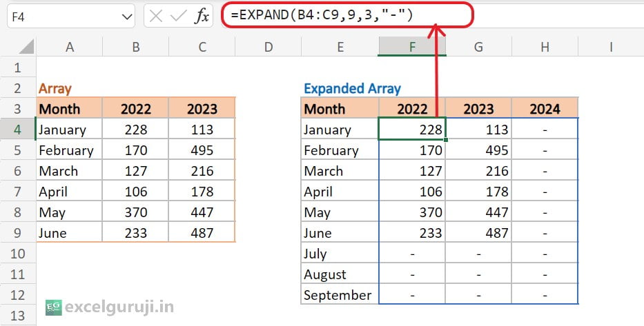
    Excel EXPAND Function Example 3

    =EXPAND(B4:C9,9,3,”-“)

    So, when you enter this formula, it takes the original array within the range B4:C9 and expands it to have 9 rows and 3 columns. The data will be repeated to meet the specified dimensions. Any empty cells in the expanded array will be filled with hyphens (“-“) as specified.

    Time to Apply What You have Learned.

    Now, it is time to put the Excel EXPAND function to the test. You can utilize the provided Excel file to experiment and witness how it operates. Inside the file, there are sample data and ready-made EXPAND formulas to kickstart your practice.

    If you have any questions or if you discover something interesting, please share your thoughts in the comments. Have fun learning by doing!

    Conclusion

    In conclusion, the Excel EXPAND function is a valuable tool for adjusting array dimensions, ensuring data consistency, and enhancing your data presentation.

    Whether you need to match array sizes, pad empty elements, or standardize your data, the EXPAND function simplifies these tasks and empowers you to work with data more efficiently.

    As with any Excel function, practice is key to mastering it. Do not hesitate to explore different applications of the EXPAND function in your own projects, and start utilizing it today to elevate your Excel skills!

    Frequently Asked Questions (FAQs)

    Q1: Can I use the EXPAND function with multiple arrays in a single formula?

    A1: The EXPAND function is designed to work with a single array. If you need to expand or pad multiple arrays, you can use the function separately for each array.

    Q2: What other Excel functions work well in conjunction with the EXPAND function?

    A2: The EXPAND function can be used in combination with various functions like IF, SUM, AVERAGE, and more, depending on your specific data processing needs.

    Q3: How do I handle errors when using the EXPAND function?

    A3: Excel returns a #VALUE error when the rows or columns argument is less than the rows or columns in the array argument. To handle errors gracefully, consider using IFERROR or other error-handling functions in your formula.

    Q4: Is it possible to expand an array with non-numeric values using the EXPAND function?

    A4: Yes, the Excel EXPAND function can be used with arrays containing both numeric and non-numeric values. It provides flexibility in handling various data types.

    Other Related Excel Functions

    Excel CHOOSE Function: A Guide to Efficient Data Selection

    Mastering Excel CHOOSECOLS Function: Custom Data Extraction and Analysis

    Join me on Instagram, YouTube and WhatApp Channel for your daily dose of valuable tips and tricks! Catch insightful videos that will enhance your knowledge and skills. Don’t miss out – follow me now!