Mastering Data Organization: A Guide to Excel SORT Function for Efficient Data Sorting

Excel SORT Function

Excel-SORT-Function

When to Use the Excel SORT Function in Excel

The SORT function1 in Excel is a powerful tool that comes in handy when you need to arrange the data in a specific order. Whether you are dealing with numerical values, dates, or text, the SORT function allows you to organize your data in ascending or descending order, making it easier to analyze and draw insights.

What Excel SORT Function Returns

The Excel SORT function returns a sorted array or range based on the specified criteria. It can be applied to both single columns and multiple columns, providing flexibility in sorting data according to your requirements.

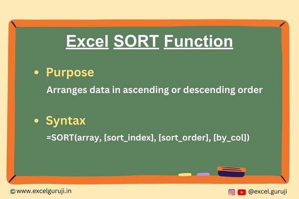
Syntax of Excel SORT Function

The syntax of the Excel SORT function is as follows:

=SORT(array, [sort_index], [sort_order], [by_col])

Input Arguments

Here are the input arguments for the Excel SORT function:

array: The range or array that you want to sort.

sort_index: (Optional) The column or row index by which to sort the array. If omitted, the function uses the first column.

sort_order: (Optional) The order in which to sort the array. Use 1 for ascending order (default) or -1 for descending order.

by_col: (Optional) A logical value that specifies whether to sort by columns (TRUE) or rows (FALSE). If omitted, the default is FALSE.

Examples of the Excel SORT Function

Here are few examples of using the Excel SORT function in Excel:

Example 1: Basic Sorting

In the following example, you will see that we have used only the first argument of the SORT function, which is an array (A2:D13)
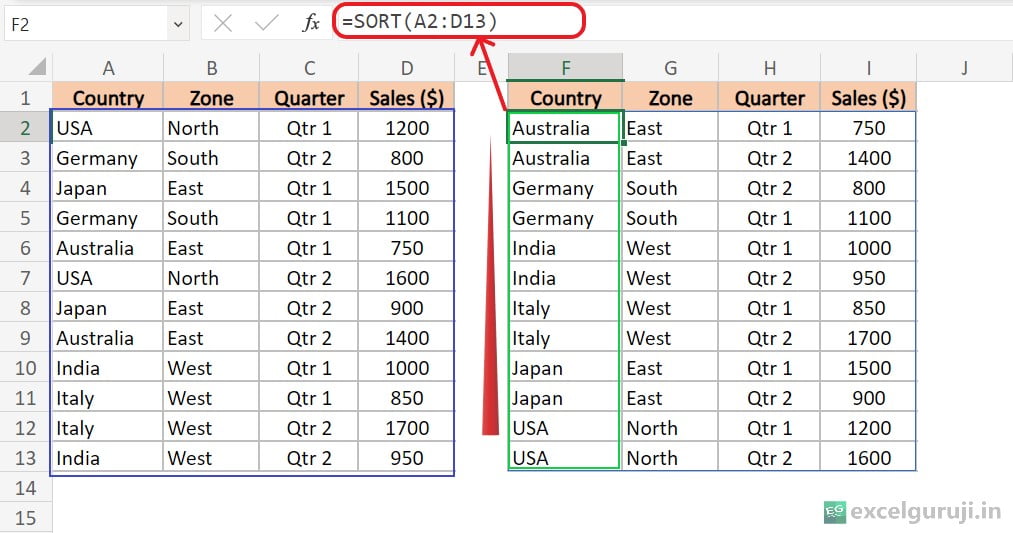
Excel-SORT-Function-Example-1-1

By default, the Excel SORT function will sort the first column of the selected array (A2:D13) in ascending order.

Example 2: Sorting by a Specific Column

As we saw in the example above, just by providing the area argument, it takes the first column and sorts it. But if you have more columns, you can sort the data by specifying the column number, The SORT function below sorts by the fourth column.
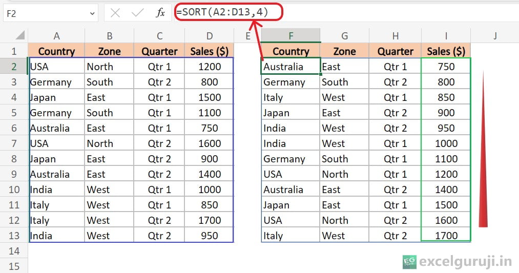
Excel-SORT-Function-Example-2-1

Note: Make changes only to the formula in cell F2. Excel will handle the rest.

Example 3: Sorting in Descending Order

Now, we use the sort_order argument (the third part of the formula) in SORT function to put the data in descending order. The formula below sorts the array based on the fourth column, from biggest to smallest.
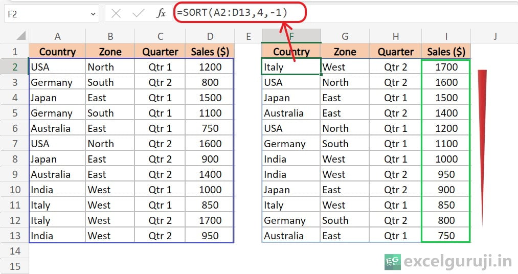
Excel SORT Function Example 3

We used -1 for the sort_order argument to arrange the data in descending order.

Example 4: Sorting on multiple columns

To sort by multiple columns, just provide an array. For example, you can sort first by Country and then by Sales.
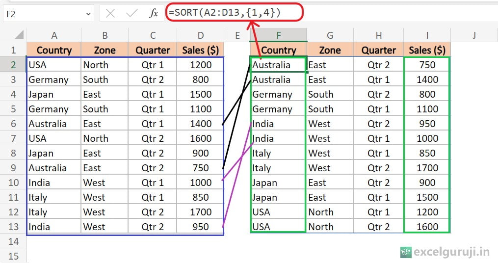
Excel-SORT-Function-Example-4

Example 5: Advanced Sorting on Multiple Columns

The advanced SORT function below showcases a sophisticated sorting approach. It begins by sorting data based on Country in ascending order, providing a primary level of organization. Subsequently, it fine-tunes the sorting criteria by incorporating Sales in descending order as a secondary parameter.
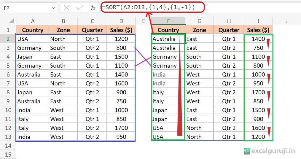
Excel-SORT-Function-Example-5

This two-step sorting process demonstrates the versatility and advanced capabilities of the SORT function in Excel.

Example 6: Conditional Sorting with Excel Filter Function

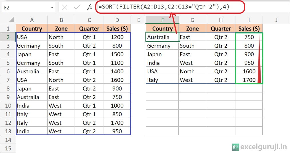
Suppose you have a dataset containing quarterly sales information for various countries in different regions, and your goal is to extract and sort data specifically for Qtr 2 sales. You can use the following formula:
Excel-SORT-Function-Example-5-2

Let’s break down the formula: =SORT(FILTER(A2:D13, C2:C13=”Qtr 2″), 4)

  • FILTER(A2:D13, C2:C13=”Qtr 2″): This part of the formula filters the data in the range A2:D13 based on the condition specified in C2:C13. It selects only the rows where the value in column C is equal to “Qtr 2”. So, it filters out the rows that don’t match the condition, effectively creating a subset of the original data.
  • SORT(…, 4): This part of the formula takes the result of the FILTER function and sorts it based on the values in the fourth column D (Sales) in ascending order by default. The number ‘4’ indicates the column number by which to sort.

Extra Notes

● Excel SORT function is exclusively accessible in Microsoft 365’s Excel and Excel for the web. It is not supported in pre-dynamic array versions of Excel (Excel 2019 and earlier) because they do not support array constants. To learn more about how to use Excel for Web for free. Watch 👇 this video

How to Get Microsoft Excel for Free | Free Microsoft Office | Microsoft Office 365

● If the sort_index argument is beyond the valid range, the SORT function returns a #VALUE! error.

● Additionally, if any cells within the spill range are not entirely blank or are merged, a #SPILL! error occurs. To resolve this issue, simply clear any obstructions in the affected cells.

Time to Apply Your Knowledge.

Take a hands-on approach to mastering the Excel FILTER function. Utilize the provided Excel file to experiment and witness its functionality with sample data.

Should you have any questions or stumble upon intriguing insights, don’t hesitate to share your thoughts in the comments. Embrace the learning journey with practical experience!

Conclusion

In conclusion, the Excel SORT function is a valuable tool for organizing and arranging data in a systematic manner. Whether you are dealing with simple lists or complex tables, the SORT function provides a versatile solution for customizing the order of your data.

Remember, exploring and experimenting with the SORT function in different scenarios will enhance your proficiency in Excel. Start incorporating the SORT function into your projects today, and streamline the way you analyze and present your data.

Frequently Asked Questions (FAQs)

Q1: Can the SORT function be used for sorting alphanumeric data?

A1: Yes, the SORT function can handle both numeric and text values, providing a comprehensive sorting solution.

Q2: Is it possible to sort data based on multiple columns?

A2: Absolutely, you can specify multiple columns for sorting.

Q3: What happens if the sort_index exceeds the number of columns in the array?

A3: If the specified sort_index is greater than the number of columns in the array, the function returns a #VALUE! error.

Q4: Can the SORT function be used to sort data in a specific order, such as a custom list?

A4: The SORT function primarily sorts data in ascending or descending order. If you need a custom sort order, additional techniques or helper columns may be required.

Q5: Does the SORT function modify the original data, or does it create a new sorted array?

A5: The SORT function returns a new array with the sorted data and does not modify the original data.

Other Related Excel Functions

Mastering Excel VLOOKUP Function: A Comprehensive Guide to Enhance Your Data Analysis Skills

Unlocking Data Mastery with Excel HLOOKUP Function: A Comprehensive Guide for Efficient Horizontal Data Lookup

Mastering Excel FILTER Function: A Comprehensive Guide for Data Filtering

Join me on Instagram, YouTube and WhatApp Channel for your daily dose of valuable tips and tricks! Catch insightful videos that will enhance your knowledge and skills. Don’t miss out – follow me now!

  1. SORT Function ↩︎

Mastering Excel OFFSET Function: A Dynamic Guide to Dynamic References

Excel OFFSET Function

Excel-OFFSET-Function

When to Use the Excel OFFSET Function in Excel

The OFFSET function1 in Excel proves to be a powerful tool when you need to dynamically reference a range of cells based on a starting point and a specified number of rows and columns. It is particularly handy for creating dynamic ranges, performing complex calculations, and building flexible data analysis models.

What Excel OFFSET Function Returns

The Excel OFFSET function returns a reference to a range that is offset from a starting reference point. The offset is determined by the specified number of rows and columns.

Syntax of Excel OFFSET Function

The syntax of the Excel OFFSET function is as follows:

=OFFSET(reference, rows, cols, [height], [width])

Input Arguments

Here are the input arguments for the Excel OFFSET function:

reference: The starting point or reference cell from which the offset will be applied. This can be a cell reference or a named range.

rows: The number of rows to offset from the reference. If you use a positive number, it moves down rows. If you use a negative number, it goes up rows. If you keep zero, then there is no change.

cols: The number of columns to offset from the reference. If you use a positive number, it moves right columns. If you use a negative number, it moves left columns. If you keep zero, then there is no change.

[height]: (Optional) The height of the range to be returned. If omitted, the function returns a single cell. Positive or negative numbers can be used; however, if you keep it as zero, a #REF! error will occur.

[width]: (Optional) The width of the range to be returned. If omitted, the function returns a single cell. Positive or negative numbers can be used; however, if you keep it as zero, a #REF! error will occur.

Learning the Basics of Excel OFFSET

The Excel OFFSET function may seem confusing at first, but once you delve into its details, you will discover its ease of use, allowing you to incorporate it systematically into your formulas.

Now, let’s explore how this function operates:

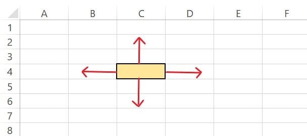
First of all, you should understand that with the help of the Excel OFFSET function, you can look up, down, left, and right.

Excel-OFFSET-Function-Example-1

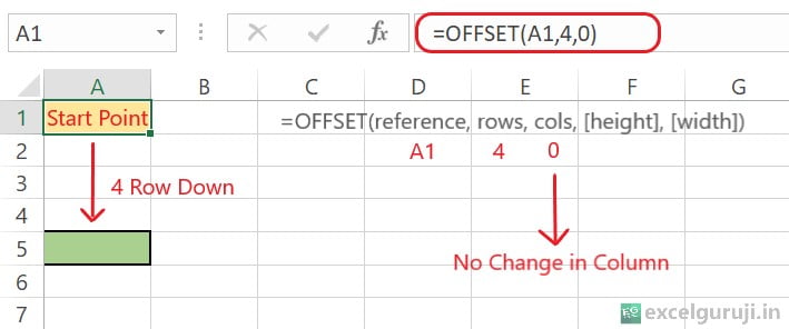
Suppose my starting point is A1, and I want to go 4 cells down. I have to write a formula like this: =OFFSET(A1,4,0)

Excel OFFSET Function Example 2

Now, let’s see how this formula works:

  • The first part (reference) decides where it starts.
  • The second part (rows), which is 4, moved down by 4 row.
  • The third part (cols), which is 0, no change in column

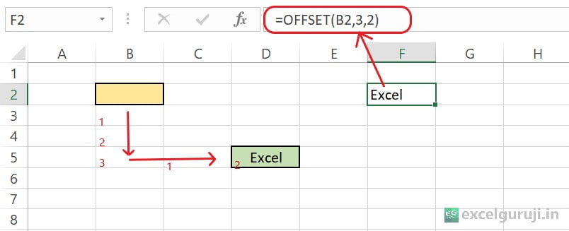
Now, suppose my starting point is the yellow cell (B2), and if I want to refer to the green cell (D5), then I have to write the formula like this.

Excel-OFFSET-Function-Example-3

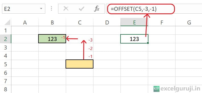
Now, let’s observe the impact by using negative values in the rows and columns arguments.

Excel-OFFSET-Function-Example-4

In the all above example, you saw how we used the necessary arguments (rows & cols) of the Excel OFFSET function. Now, let’s check out how to use the optional [height] and [width] arguments.

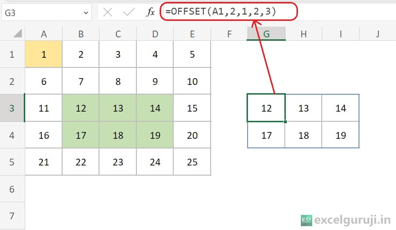
Imagine you want to use cell A1 (highlighted in yellow) as the reference and refer to the entire highlighted range in green (B3:D4) within a formula.

Excel-OFFSET-Function-Example-5-1

Now, let’s see how this formula works:

  • The first part (reference) decides where it starts, which, in this case, is cell A1.
  • The second part (rows), which is 2, moved down by 2 row.
  • The third part (cols), which is 1, moved right by 1 column.
  • The fourth part [height], which is 2, cover 2 rows.
  • The fifth part [width], which is 3, cover 3 columns.

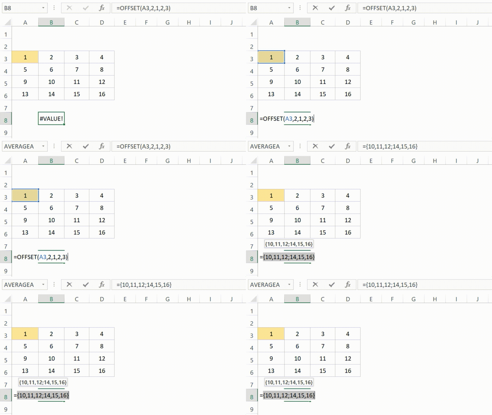
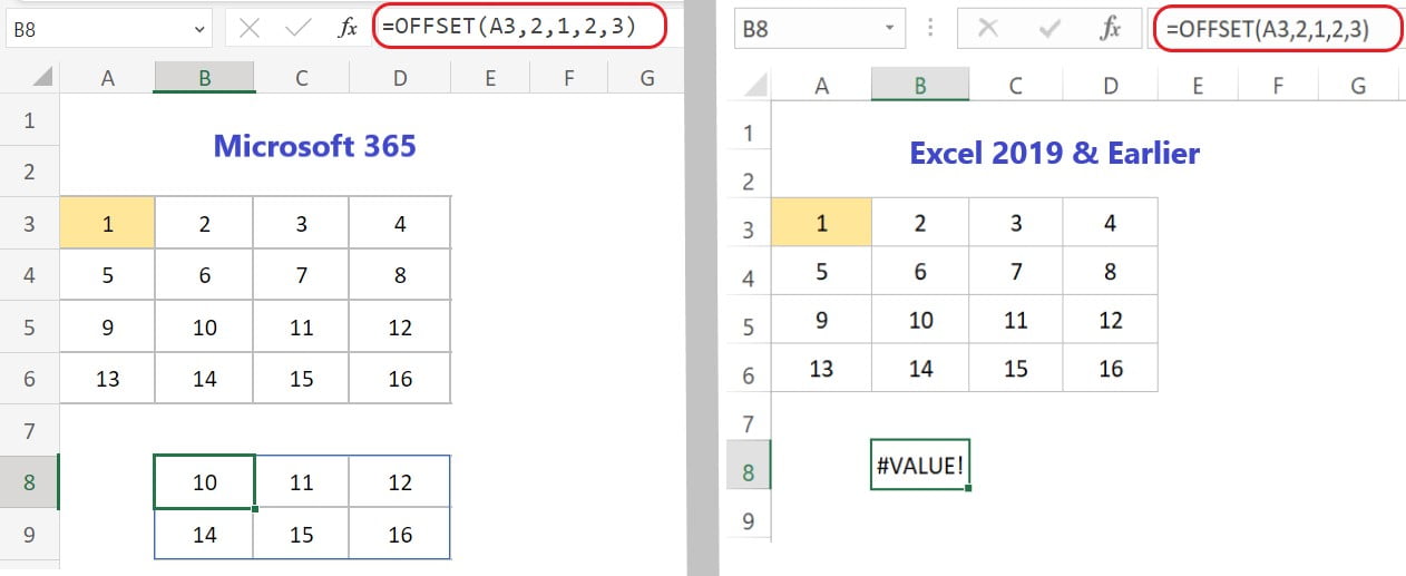
Note : It is important to note that if you are using a pre-dynamic array version (Excel 2019 and earlier), and you use the height and row arguments, you will encounter a #VALUE! error.

Excel-OFFSET-Function-Example-6

But don’t worry, you can still use the OFFSET function along with other functions even if there is an error. Just go to the cell’s edit mode, press F9, and you will see it gives you all the values it refers to in the formula.

OFFSET

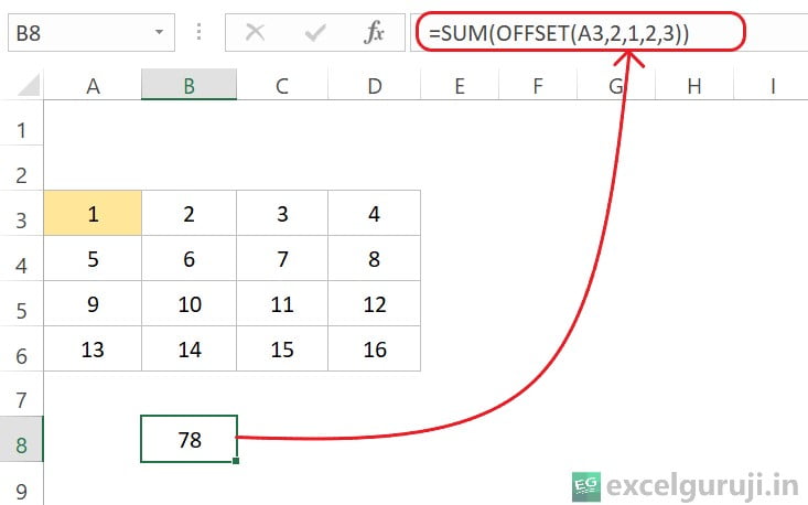
Now, let’s say you want to add up all these values. You can easily do this by using the SUM function.

Excel-OFFSET-Function-Example-7

Hopefully, now you have a good idea of how to use the Excel OFFSET function. Let’s check out some real-life examples to make it even clearer.

Examples of the Excel OFFSET Function

Here are few examples of using the Excel OFFSET function in Excel:

Example 1: Find the Last Filled Cell

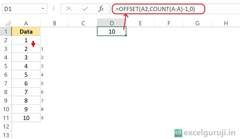
Imagine you have a list of numbers in column A, and you want to dynamically find the last filled cell in that column. Let’s explore how you can achieve this using the OFFSET function.

Excel OFFSET Function Example 8

Here is an explanation of the formula: =OFFSET(A2,COUNT(A:A)-1,0)

  • A2: This is the starting reference point for the OFFSET function. It begins counting from cell A2.
  • COUNT(A:A)-1: This part determines the number of non-empty cells in column A. COUNT(A:A) counts all the cells in column A that have numbers in them. Subtracting 1 (-1) adjusts for the starting point A2. If you have numbers in cells A2 to A11, COUNT(A:A)-1 would be 10 – 1 = 9.
  • 0: This is the number of columns to move to the right from the starting point (A2). Since it is 0, the OFFSET function stays in the same column.

Example 2: Drop Down that Adjusts Dynamically

You can apply the principles demonstrated in Example 1 to expand upon the idea and generate a dynamically adjusting drop-down list.

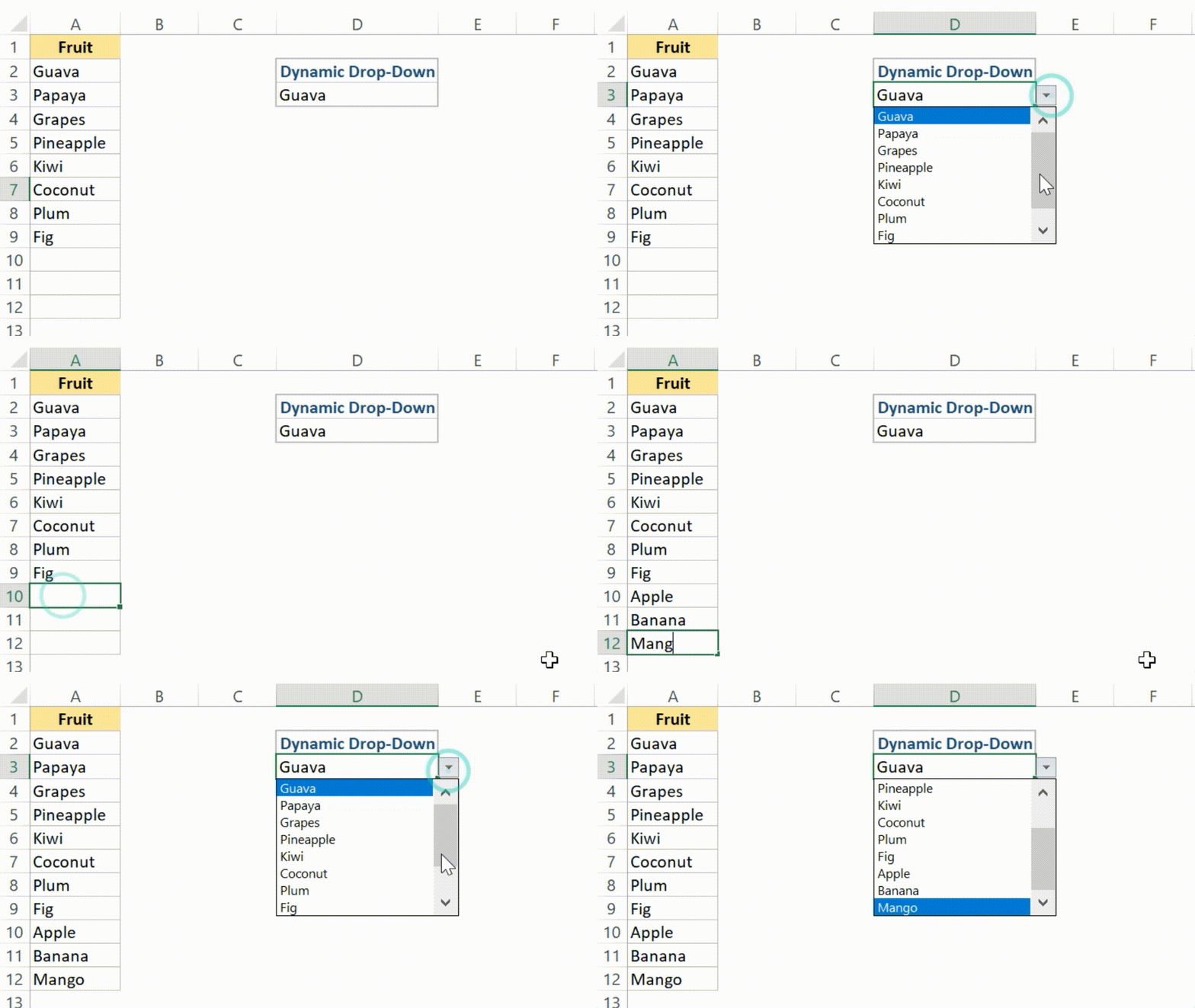
Imagine you are tasked with managing inventory of different fruits. And you want to create a dynamic drop-down list, and it automatically adjusts as you add or remove fruits name from the list in column A.

Here is an example of how it works:

OFFSET-Drop-Down

This happens because the formula used to make the drop-down is dynamic. It can figure out if you add or remove something and then adjust itself.

Here is how to make it work:

  • Select the cell where you want the drop-down.
  • Go to Data –> Data Tools –> Data Validation.
Excel OFFSET Function Example 9
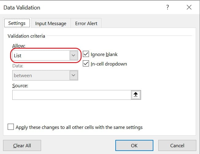
  • In the Data Validation box, choose List from the options.
Excel OFFSET Function Example 10
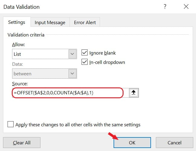
  • In the source, type this formula: =OFFSET($A$2,0,0,COUNTA($A:$A),1), and Click OK
Excel OFFSET Function Example 11

Let’s understand how this formula works:

  • $A$2: This is the starting reference cell. The OFFSET function will use this cell as the starting point for the dynamic range.
  • 0,0: These are the row and column offsets. In this case, both are set to 0, meaning there is no offset from the starting cell. The dynamic range starts from the cell specified in $A$2.
  • COUNTA($A:$A): This part calculates the height of the range. COUNTA($A:$A) counts the number of non-empty cells in column A. It dynamically adjusts as you add or remove items from column A.
  • 1: This represents the width of the range. In this case, it is set to 1, indicating that the dynamic range is one column wide.

Extra Notes

● Excel OFFSET function is a volatile functions (functions that recalculate with every change in the worksheet). This lead to performance issues and slow down your workbook.

● If the specified number of rows or columns is negative, the OFFSET function will reference cells above or to the left of the starting point.

● If the [height] and [width] arguments are omitted, the function returns a reference to a single cell.

● If the rows and columns offset the reference beyond the edge of the worksheet, OFFSET will show #REF! error.

● OFFSET doesn’t physically move cells or alter the selection, it simply gives a reference. You can pair OFFSET with any function that needs a reference.

Practice Workbook

Download Free Excel File For Practice

Conclusion

In conclusion, the Excel OFFSET function is a versatile and powerful tool for dynamic referencing and data extraction. Whether you are building dynamic ranges, creating flexible models, or navigating through datasets, the OFFSET function can significantly enhance your Excel capabilities.

Remember, as with any Excel function, understanding its use and practicing in different scenarios will help you master the OFFSET function. Start incorporating OFFSET into your Excel toolkit today and open up new possibilities for dynamic data analysis.

Frequently Asked Questions (FAQs)

Q1: Can the Excel OFFSET function be used to reference a range from another sheet?

A1: Yes, the Excel OFFSET function can reference ranges from other sheets within the same workbook.

Q2: What happens if the specified rows or columns go beyond the boundaries of the worksheet?

A2: If the offset goes beyond the boundaries, Excel will return a #REF! error.

Q3: Can the OFFSET function be combined with other functions for advanced data analysis?

A3: Absolutely, the OFFSET function can be combined with various other functions, such as SUM, COUNT, AVERAGE, IF, etc. for advanced data analysis and modeling.

Q4: Are there any alternatives to the Excel OFFSET function for dynamic range creation?

A4: Yes, other functions like INDEX and INDIRECT can also be used for dynamic range creation, depending on the specific requirements of your workbook.

Other Related Excel Functions

Mastering Excel INDEX Function: A Guide to Dynamic Data Retrieval and Manipulation

Unleashing the Power of Excel INDIRECT Function: A Comprehensive Guide to Dynamic Cell Referencing

Mastering Excel VLOOKUP Function: A Comprehensive Guide to Enhance Your Data Analysis Skills

Unlocking Data Mastery with Excel HLOOKUP Function: A Comprehensive Guide for Efficient Horizontal Data Lookup

Mastering Excel FILTER Function: A Comprehensive Guide for Data Filtering

Join me on Instagram, YouTube and WhatApp Channel for your daily dose of valuable tips and tricks! Catch insightful videos that will enhance your knowledge and skills. Don’t miss out – follow me now!
  1. OFFSET Function ↩︎

Unleashing the Power of Excel INDIRECT Function: A Comprehensive Guide to Dynamic Cell Referencing

Excel INDIRECT Function

Excel-INDIRECT-Function

When to Use the Excel INDIRECT Function in Excel

The INDIRECT function1 in Excel proves invaluable when you need to dynamically reference cells or ranges. It allows you to create flexible and dynamic formulas by converting text representations of cell references or named ranges into actual references.

What Excel INDIRECT Function Returns

The Excel INDIRECT function returns the value of the referenced cell or range specified by a text string. This enables you to construct formulas that can change dynamically based on the contents of a cell.

Syntax of Excel INDIRECT Function

The syntax of the Excel INDIRECT function is as follows:

=INDIRECT(ref_text, [a1])

Input Arguments

Here are the input arguments for the Excel INDIRECT function:

ref_text: This is the reference text that you want to convert into an actual cell reference or a named range. It can be a text string enclosed in quotation marks, a cell reference, or the result of another formula.

[a1]: This is an optional argument that determines the reference type. If omitted or set to TRUE, the reference is interpreted in A1 style (column letter and row number). If set to FALSE, the reference is interpreted in R1C1 style (row and column number).

Excel INDIRECT Function

Extra Notes

● If the ref_text argument refers to a cell on another sheet, that sheet must be open, or the INDIRECT function will return a #REF! error.

● Excel INDIRECT function is a volatile functions (functions that recalculate with every change in the worksheet). This lead to performance issues and slow down your workbook.

● The ref_text argument can include the sheet name followed by an exclamation mark to specify a cell or range on a different sheet.

Examples of the Excel INDIRECT Function

Here are few examples of using the Excel INDIRECR function in Excel:

Example 1: Basic Usage

Suppose you have data in cell A1, and you want to retrieve the value from that cell using the INDIRECT function. You just need to provide it with the name of the cell, written as text, as shown in the example below.

Excel-INDIRECT-Function-Example-1

Here is an explanation of the formula: =INDIRECT(“A1”)

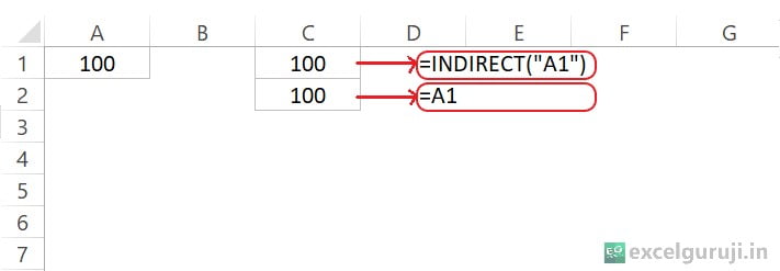
The formula above accepts the cell reference A1 as an input argument (enclosed in double quotes as a text string) and yields the value found in that cell, which, in this case, is 100.

Now, you might be wondering if this could have been achieved by directly referencing the sales (e.g., A1 or =$A$1), as demonstrated below. Then, why should we use the INDIRECT function unnecessarily?

Excel-INDIRECT-Function-Example-2

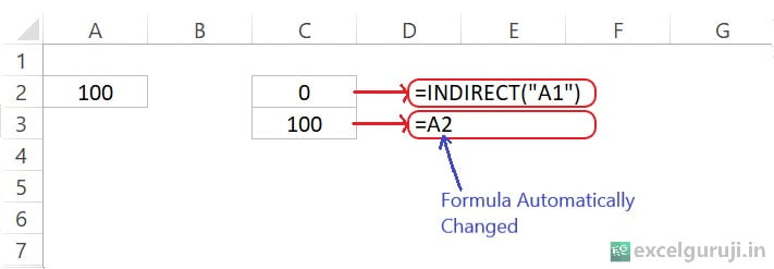
When you use =A1 or =$A$1, you get the same result. But, if you add a row above the first row, the cell references change automatically to fit the new row.

Excel-INDIRECT-Function-Example-3

When adding rows or columns to a worksheet and needing to keep the cell reference locked and unchanged, you can utilize the Excel INDIRECT function.

Example 2: Use Cell Reference

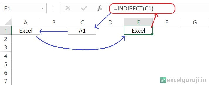
Suppose you have data in cell A1, and you want to dynamically reference the cell specified in cell C1. In cell E1, you can use the following formula:

Excel-INDIRECT-Function-Example-4

When you use the Excel INDIRECT function with C1 (which holds a cell address as text), it makes A1 a proper reference. This means it looks at A1 and gives you what is there.

Remember, no need for quotes because C1 has the cell address in text.

But if C1 has something that is not a proper cell address, INDIRECT will show an error (#REF!).

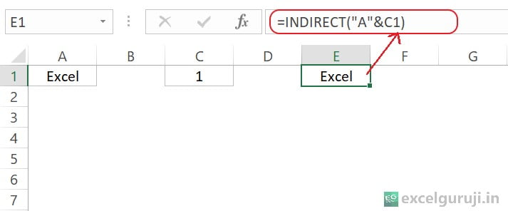
You can make a reference to a cell by using both the column letter and the row number. For example, if you have the number 1 in cell C1, and you use the formula =INDIRECT(“A” & C1), it will point to cell A1, as shown in the example below.

Excel-INDIRECT-Function-Example-5

Example 3: Calculate the Average of a Range of Cells

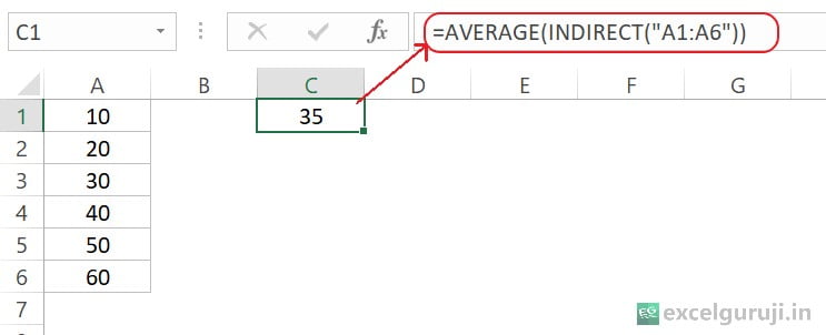
You can use the Excel INDIRECT function in Excel to reference a range of cells, just as you would reference a single cell, as shown in the example below.

Excel-INDIRECT-Function-Example-6

Here is an explanation of the formula: =AVERAGE(INDIRECT(“A1:A6”))

  • INDIRECT(“A1:A6”): The INDIRECT function is used to convert the text string “A1:A6” into a reference to the actual range A1 to A6. So, it essentially refers to the range of cells A1 to A6.
  • AVERAGE(INDIRECT(“A1:A6”)): The AVERAGE function then calculates the average of the numbers in the range A1 to A6.

Just like the AVERAGE function, you can use other functions such as SUM, COUNT, MAX, MIN, LARGE, SMALL, etc.

Example 4: INDIRECT Function With Name Range

When Excel INDIRECT function combined with named ranges, it can be a powerful tool for creating dynamic and flexible formulas. Named ranges allow you to assign a meaningful name to a specific cell or range of cells, making it easier to understand and manage your formulas.

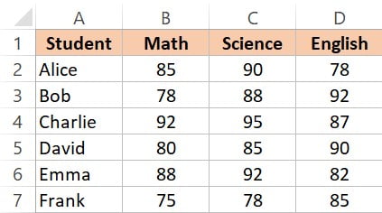
Suppose you have the following data on test scores for students in different subjects:

Excel INDIRECT Function Example 7 1

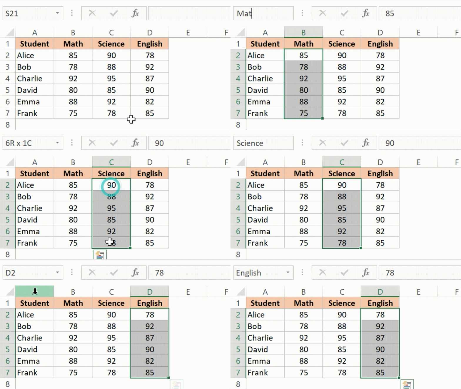
The scores for the subjects are listed in columns B, C, and D. To make it easier to refer to these ranges, you can assign names to them. Specifically, you want to name the range in column B as “Math” the range in column C as “Science”, and the range in column D as “English”.

Now, to achieve this, you can follow the method below:

Select the Range:

  • Highlight the cells in column B where the Math scores are (e.g., B2 to B7).
  • Then, go to the “Formulas” tab on the ribbon.
  • Click on “Define Name” or “Name Manager” (depending on your Excel version).
  • Enter the name “Math” and click OK. Now, the range B2:B7 is named as “Maths”.
  • Repeat the same process for Other Subjects:
Indirect-Function-1

Now, you can use the Excel INDIRECT function to refer to the named range in a formula.

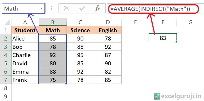
For example, if you want to average the values in the named range “Math” you could use the following formula:

Excel-INDIRECT-Function-Example-8

Example 5: Dependent Drop-down List with the Excel INDIRECT Function

Creating a dependent dropdown list in Excel using the INDIRECT function involves setting up named ranges and using data validation.

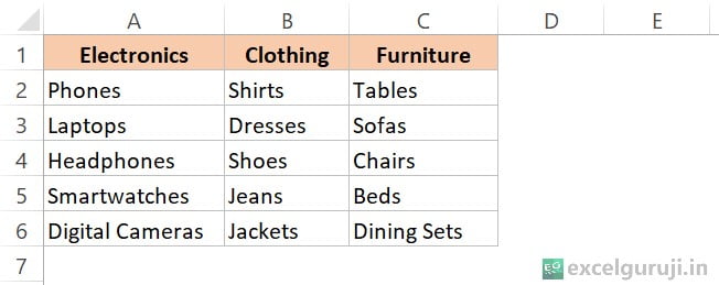
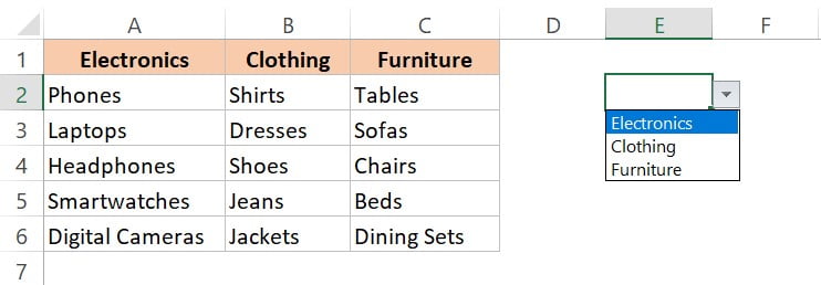
For example, suppose you have a list of categories arranged in a row and their corresponding subcategories in a column, as shown below:

Excel-INDIRECT-Function-Example-9

Now, to create a dependent dropdown list, assign a name range to each category, such as A2:A6 for Electronics, B2:B6 for Clothing, and C2:C6 for Furniture. We have already covered how to assign name ranges in the previous example.

Now, select the cell where you want to create a dropdown list for the main category (Electronics, Clothing, Furniture). This will be the first drop-down list.

  • Select cell E2
  • Click on Data Tab
  • Click on Data Validation
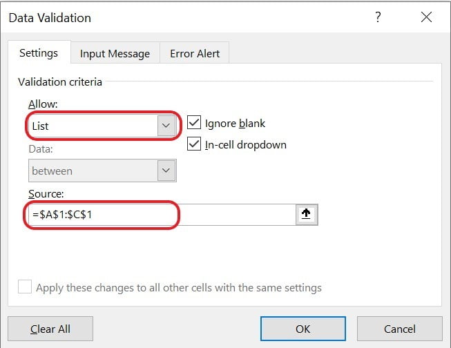
  • Select List as the Validation criteria and use the following formula in the Source field: =$A$1:$C$1
Excel-INDIRECT-Function-Example-10-1

Your first drop-down list will look like below:

Excel-INDIRECT-Function-Example-11

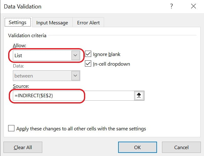
Now follow below method to create dependable drop-down list:

  • Select cell F2
  • Click on Data Tab
  • Click on Data Validation
  • Select List as the Validation criteria and use the following formula in the Source field: =$A$1:$C$1
Excel-INDIRECT-Function-Example-12

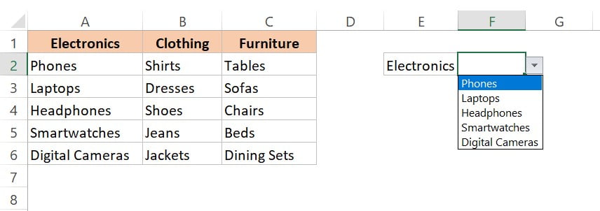
Now, when you select ‘Electronics’ in the first drop-down (cell E2), the dependent drop-down in cell F2 will display the subcategories of Electronics (Phones, Laptops, Headphones, Smartwatches, Digital Cameras).

Excel INDIRECT Function Example 13

And when you select ‘Furniture’ in the first drop-down, the dependent drop-down in cell F2 will display the subcategories of Furniture (Tables, Sofas, Chairs, Beds, Dining Sets).

Practice Workbook

Download Free Excel File For Practice

Conclusion

In conclusion, the Excel INDIRECT function is a powerful tool for creating dynamic and flexible formulas. It enables you to build formulas that adapt to changes in your spreadsheet, providing a level of versatility that static cell references cannot achieve.

As with any Excel function, it is essential to understand the nuances and potential pitfalls of the INDIRECT function. Experiment with different applications to enhance your proficiency and efficiency in utilizing this function in your Excel projects.

Frequently Asked Questions (FAQs)

Q1: Can the INDIRECT function reference cells on other sheets?

A1: Yes, by including the sheet name followed by an exclamation mark in the ref_text argument.

Q2: What happens if the referenced sheet is not open?

A2: If the referenced sheet is not open, the INDIRECT function will return a #REF! error.

Q3: What is the purpose of the [a1] argument?

A3: The [a1] argument determines the reference type. If TRUE or omitted, the reference is interpreted in A1 style; if FALSE, in R1C1 style.

Q4: Is there a performance impact when using the INDIRECT function with volatile functions?

A4: Yes, using the INDIRECT function with volatile functions can lead to performance issues.

Other Related Excel Functions

Mastering Excel VLOOKUP Function: A Comprehensive Guide to Enhance Your Data Analysis Skills

Unlocking Data Mastery with Excel HLOOKUP Function: A Comprehensive Guide for Efficient Horizontal Data Lookup

Mastering Excel FILTER Function: A Comprehensive Guide for Data Filtering

Join me on Instagram, YouTube and WhatApp Channel for your daily dose of valuable tips and tricks! Catch insightful videos that will enhance your knowledge and skills. Don’t miss out – follow me now!
  1. Indirect Function ↩︎

Mastering Excel MATCH Function: A Comprehensive Guide to Efficient Data Lookup

Excel MATCH Function

Excel-MATCH-Function

When to Use the Excel MATCH Function in Excel

The MATCH function1 in Excel comes in handy when you need to:

Locate the position of a specific value in a range.
Check if a value exists in a list or array.
Determine the relative position of an item in a sorted or unsorted list.

What Excel MATCH Function Returns

The Excel MATCH function returns the relative position of a specified value in a range. The result can be one of three values:

● If the function finds an exact match, it returns the position of the item.
● If no match is found, it returns the #N/A error.
● If the match type is set to 1 and the data is not sorted, it returns the position of the nearest value less than or equal to the lookup value.

Syntax of Excel MATCH Function

The syntax of the Excel MATCH function is as follows:

=MATCH(lookup_value, lookup_array, [match_type])

Input Arguments

Here are the input arguments for the Excel MATCH function:

lookup_value: The value you want to find in the lookup_array.

lookup_array: The range of cells containing possible matches.

match_type: An optional argument that specifies the type of match. It can be 1 (less than), 0 (exact match), or -1 (greater than).

Match Type Behavior:

  • 1 or Omitted: If no exact match is found, the function returns the position of the closest value less than the lookup value. The lookup array must be sorted in ascending order.
  • 0: If no exact match is found, the function returns an error. The lookup array does not need to be sorted.
  • -1: If no exact match is found, the function returns the position of the closest value greater than the lookup value. The lookup array must be sorted in descending order.

Extra Notes

● MATCH is not case-sensitive.

● When no match is found, MATCH returns the #N/A error.

● MATCH is limited to working with text strings of up to 255 characters in length.

● If there are duplicate values, MATCH returns the position of the first occurrence.

● For match_type values of -1 or 1, it is essential for the lookup_array to be sorted, as mentioned earlier.

Examples of the Excel MATCH Function

Here are few examples of using the Excel MATCH function in Excel:

Example 1: Basic Usage

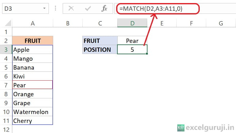
Suppose you have a list of fruits names in column A, and you want to find the position of the fruit “Pear” in the list. In cell D3, use the following formula:

Excel-MATCH-Function-Example-1

Here is an explanation of the formula: =MATCH(D2,A3:A11,0)

  • D2: This is the lookup_value. In this case, it is “Pear”, and the formula is trying to find the position of “Pear” within the specified range.
  • A3:A11: This is the lookup_array. It represents the range of cells where Excel will search for the value “Pear”.
  • 0: This is the match_type. The value 0 indicates that the function should find an exact match.

Example 2: Less Than Match

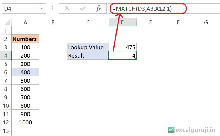
Suppose you have a set of numbers, and you want to find the position of the largest number less than the given lookup value. So, you need to select 1 for the match_type argument and write the MATCH function as shown below:

Excel MATCH Function Example 2

So, in the above example, we observe that the largest value below lookup_value (475), i.e., the number 400, is located at the fourth position. As mentioned earlier, we have arranged the lookup_array (A3:A12) in ascending order (smallest to largest) to obtain the correct result.

Example 3: Greater Than Match

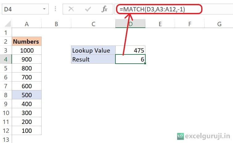
Suppose you have a set of numbers, and you want to find the position of the smallest number greater than a given lookup value. So, you need to select -1 for the match_type argument and write the MATCH function as shown below:

Excel MATCH Function Example 3

So, in the above example, we observe that the smallest value above lookup_value (475), i.e., the number 500, is located at the sixth position. As mentioned earlier, we have arranged the lookup_array (A3:A12) in descending order (largest to smallest) to obtain the correct result.

Example 4: INDEX Function With MATCH Function

INDEX Function and MATCH Function are like a dynamic duo in Excel. They team up to search for data in a flexible way. They don’t mind how the columns are arranged, can hunt for data in both rows and columns, easily adapt to different criteria, handle unsorted data well, manage errors gracefully, and can be used as array formulas. This makes them versatile and powerful tools for handling various data situations in Excel.

I highly recommend reading my previous INDEX function post for a deeper understanding of this concept.

Practice Workbook

Download Free Excel File For Practice

Conclusion

In conclusion, the Excel MATCH function is a valuable tool for locating specific values in a range. Whether you are working with lists of data, managing inventories, or analyzing information, the MATCH function can streamline your tasks and improve your Excel proficiency.

As with any Excel function, it’s essential to understand the syntax and experiment with different scenarios to master its usage. Start incorporating the MATCH function into your Excel projects today to enhance your data analysis and decision-making capabilities.

Frequently Asked Questions (FAQs)

Q1: Can the MATCH function be used to find the position of the last occurrence of a value?

A1: No, the MATCH function returns the position of the first occurrence of a value.

Q2: Is the MATCH function case-sensitive?

A2: No, the MATCH function is not case-sensitive.

Q3: What does the #N/A error mean in the context of the MATCH function?

A3: The #N/A error is returned when no match is found for the specified lookup value.

Q4: Can the Excel MATCH function handle arrays as lookup arrays?

A4: Yes, the Excel MATCH function can handle arrays as lookup arrays, making it versatile for various data structures.

Other Related Excel Functions

Mastering Excel VLOOKUP Function: A Comprehensive Guide to Enhance Your Data Analysis Skills

Unlocking Data Mastery with Excel HLOOKUP Function: A Comprehensive Guide for Efficient Horizontal Data Lookup

Mastering Excel FILTER Function: A Comprehensive Guide for Data Filtering

Join me on Instagram, YouTube and WhatApp Channel for your daily dose of valuable tips and tricks! Catch insightful videos that will enhance your knowledge and skills. Don’t miss out – follow me now!
  1. Match Function ↩︎

Mastering Excel INDEX Function: A Guide to Dynamic Data Retrieval and Manipulation

Excel INDEX Function

Excel-INDEX-Function

When to Use the Excel INDEX Function in Excel

The INDEX function1 in Excel is a versatile tool designed for retrieving data from specific locations within a range, array, or reference. It offers dynamic solutions for data manipulation, making it an invaluable asset in scenarios where you need to work with tables, lists, or multiple ranges.

What Excel INDEX Function Returns

The Excel INDEX function returns the value of a cell in a specified range, array, or reference based on the row and column numbers provided as arguments.

Syntax of Excel INDEX Function

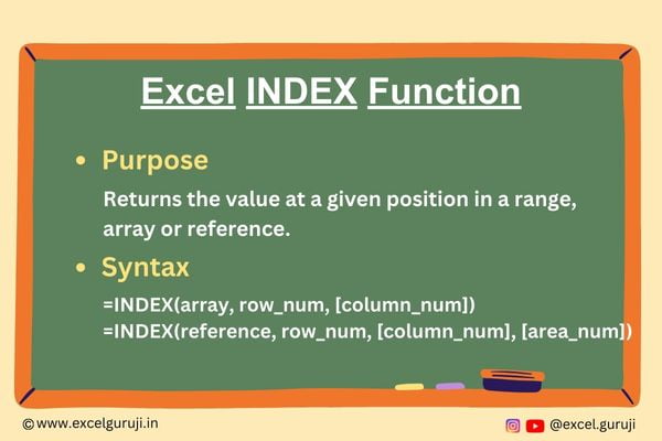
The Excel INDEX function has two syntax variations, depending on the type of data source:

Syntax 1: Syntax for Array or Range

=INDEX(array, row_num, [column_num])

This syntax is designed for situations where you are working with a single range or array of data.

Syntax 2: Syntax for Reference with Multiple Areas:

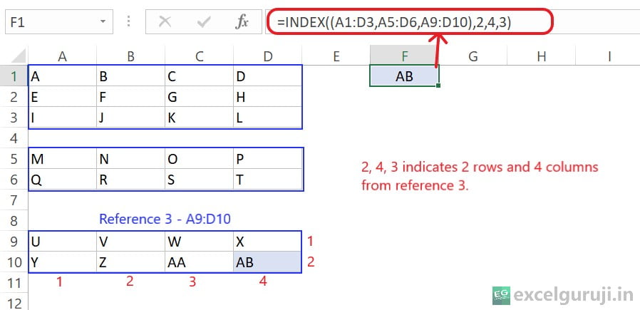
=INDEX(reference, row_num, [column_num], [area_num])

This syntax is intended for cases where your data is organized into multiple non-contiguous ranges or areas. It enables you to reference a broader scope that consists of multiple areas, allowing you to retrieve data from specific rows and columns within those areas.

Input Arguments

Here are the input arguments for both variations of the Excel INDEX function:

array: The range of cells, table, or array from which you want to retrieve the data.

reference: The reference to a range that may consist of multiple areas. Such as (A1:C10, D7:F15).

row_num: The row number within the reference from which to retrieve the data. It must be a positive integer.

column_num: [Optional] The column number within the reference from which to retrieve the data. It must be a positive integer

Note: If you are using the Microsoft 365 version, setting the row_num & column_num argument to zero or leaving it blank (Omitted) will provide all rows and columns in the default array. However, in pre-dynamic array Excel (2019 and lower), you will receive a #VALUE! error in response.

Excel-INDEX-Function-Syntax

area_num: [Optional] The number of the area in reference from which to retrieve the data. If omitted, the function defaults to the first area.

Excel-INDEX-Function-Syntax-2

Extra Notes

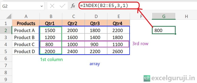
● If both row_num and column_num are provided, the function returns the value at the intersection of the specified row and column.

● If only row_num is provided, the function returns the entire row specified by that number (Only in the 365 version, the error will occur in the previous versions).

● If only column_num is provided, the function returns the entire column specified by that number (Only in the 365 version, the error will occur in the previous versions).

#VALUE! error takes place when any of the provided row_num, column_num, or area_num arguments are non-numeric.

● It is essential that row_num and column_num and area_num arguments point to a cell within the array, otherwise, INDEX returns a #REF! error.

● If the array consists of only one row or column, the corresponding row_num or column_num argument becomes optional.

● In the scenario where the array has more than one row and more than one column, and only row_num or column_num is utilized, INDEX returns an array comprising the entire row or column in the array (Only in the 365 version, the error will occur in the previous versions).

Examples of the Excel INDEX Function

Here are few examples of using the Excel INDEX function in Excel:

Example 1: Basic Usage

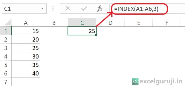
The Excel INDEX function retrieves a specific value from a range of cells based on its position. If the range is a single column or row, only a row or column number is required. However, for a two-dimensional range, both row and column numbers are necessary. You would use the formula like the following.

Excel-INDEX-Function-Example-11-1

Now, The following formulas demonstrate how the Excel INDEX function can be employed to retrieve a value from a two-dimensional range:

Excel-INDEX-Function-Example-1

Example 2: INDEX Function With MATCH Function

INDEX function and MATCH function are often used together in Excel due to their flexibility in dynamic data lookup, independence from column order, support for two-dimensional lookups, improved flexibility in changing lookup criteria, effectiveness with unsorted data, error handling capabilities, and the ability to function as array formulas, making them versatile tools in various data scenarios.

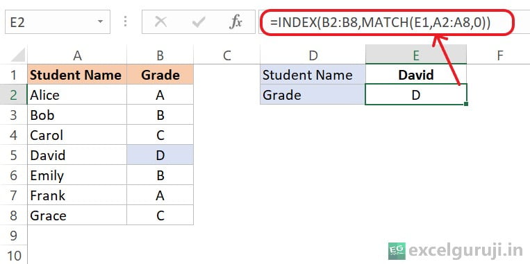
Suppose you have data on students and their grades, and you want to extract the grade with the help of the INDEX and MATCH functions. You can use the following formula:

Excel-INDEX-Function-Example-2

Here is an explanation of the formula: =INDEX(B2:B8,MATCH(E1,A2:A8,0))

  • INDEX(B2:B8): This part of the formula refers to the range of grades (A, B, C, etc.), which is in column B from row 2 to row 8.
  • MATCH(E1, A2:A8, 0): This part of the formula looks for the position of the value in cell E1 (which is “David” in this case) within the range A2:A8. The 0 in the MATCH function indicates an exact match.
  • The MATCH function returns the relative position of the value in cell E1 within the range A2:A8. In this case, it returns 4 because “David” is in the fourth position in the list.
  • Finally, INDEX uses this position (4) to retrieve the corresponding value from the range B2:B8, which is the grade associated with “David”. In your case, the grade is “D”.

So, the overall formula is finding the grade associated with the student name “David” and placing it in cell E2. If you change the value in cell E1 to another student name, the formula will dynamically retrieve the corresponding grade for that student.

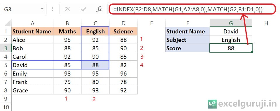
In the above example, we used the MATCH function in place of the row_num argument. In the following example, we use the MATCH function in place of both the row_num and column_num arguments.

Excel-INDEX-Function-Example-3

Here is an explanation of the formula: =INDEX(B2:D8,MATCH(G1,A2:A8,0),MATCH(G2,B1:D1,0))

  • MATCH(G1, A2:A8, 0): Matches “David” in the range A2:A8, and returns the row position. In this case, it returns 4 because “David” is in the fourth row.
  • MATCH(G2, B1:D1, 0): Matches “English” in the range B1:D1, and returns the column position. Here, it returns 2 because “English” is in the second column.
  • INDEX(B2:D8, …, …): Uses the row and column positions obtained from the MATCH functions to index into the data range B2:D8. So, the final formula looks like this =INDEX(B2:D8,4,2)

Therefore, the formula returns the score of David in English, which is the value at the intersection of the fourth row and second column in the range B2:D8. In this case, it is 88.

Practice Workbook

Download Free Excel File For Practice

Conclusion

In conclusion, the Excel INDEX function, with its two syntax variations, is a powerful tool for dynamic data retrieval and manipulation. Whether you are working with single arrays or referencing multiple areas across sheets, the Excel INDEX function provides a flexible solution for extracting specific data points based on specified criteria.

As you integrate the Excel INDEX function into your projects, you will find its versatility and functionality enhance your ability to handle diverse datasets and streamline your Excel workflows.

Frequently Asked Questions (FAQs)

Q1: Can the INDEX function retrieve data from multiple sheets?

A1: Yes, the INDEX function can be used to retrieve data from multiple sheets by referencing the appropriate sheet in the array argument.

Q2: Can the INDEX function handle non-numeric data?

A2: Absolutely, the INDEX function can handle both numeric and non-numeric data, making it suitable for various types of datasets.

Q3: What happens if the specified row or column number is outside the range of the array?

A3: If the specified row or column number is outside the range, the function may return an error.

Q4: Can the INDEX function be combined with other functions for more complex data manipulation?

A4: Yes, the INDEX function can be combined with other Excel functions to create more complex formulas for advanced data manipulation.

Q5: Is the INDEX function case-sensitive when working with text data?

A5: No, the INDEX function operates in a case-insensitive manner when working with text data.

Other Related Excel Functions

Mastering Excel VLOOKUP Function: A Comprehensive Guide to Enhance Your Data Analysis Skills

Unlocking Data Mastery with Excel HLOOKUP Function: A Comprehensive Guide for Efficient Horizontal Data Lookup

Mastering Excel FILTER Function: A Comprehensive Guide for Data Filtering

Join me on Instagram, YouTube and WhatApp Channel for your daily dose of valuable tips and tricks! Catch insightful videos that will enhance your knowledge and skills. Don’t miss out – follow me now!
  1. Index Function ↩︎

Mastering Excel: Unleashing the Power of the Excel MAX Function for Data Analysis

Excel MAX Function

Excel-MAX-Function

When to Use the Excel MAX Function in Excel

The MAX function in Excel is a powerful tool used to find the highest value within a range of numbers. Whether you are dealing with financial data, analyzing test scores, or managing project timelines, the MAX function can quickly identify the maximum value, providing valuable insights into your dataset.

What Excel MAX Function Returns

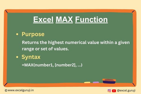
The Excel MAX function returns the highest value from a set of values.

Syntax of Excel MAX Function

The syntax of the Excel MAX function is as follows:

=MAX(number1, [number2], …)

Input Arguments

Here are the input arguments for the Excel MAX function:

number1, [number2], …: These are the numerical values or ranges for which you want to find the maximum. You can input up to 255 arguments. The number1 argument is compulsory; others are optional.

Extra Notes

● Non-numeric values, logical values, and text representations of numbers are ignored.

● If all the arguments are empty, the function returns a 0.

● If MAX function encounters an error within a range, it will output an error.

Examples of the Excel MAX Function

Here are few examples of using the MAX function in Excel:

Example 1: Basic Usage

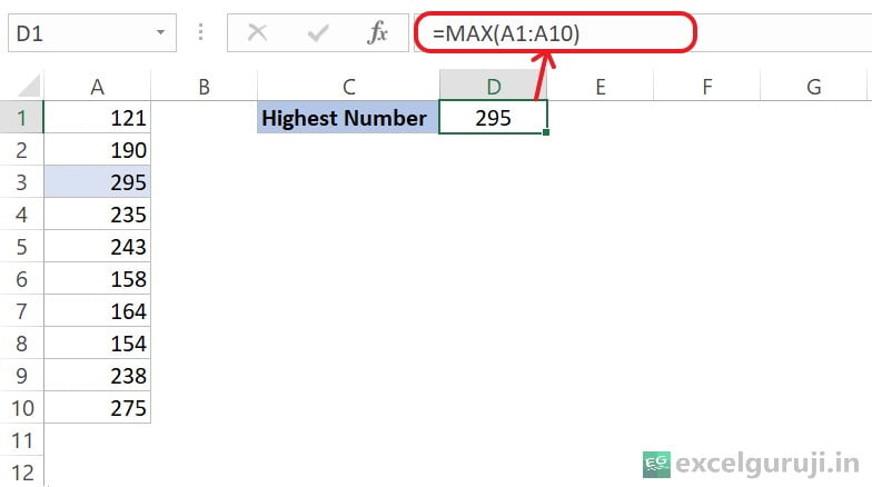
Suppose you have a dataset in cells A1 to A10, and you want to find the highest value. In cell D1, use the following formula:

Excel-MAX-Function-Example-1

This will return the highest value in the range.

Example 2: Using Multiple Ranges

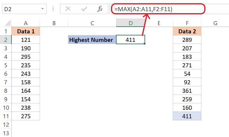
If your dataset is split across different columns, and you want to find the overall maximum, you can use the MAX function with multiple ranges:

Excel-MAX-Function-Example-2

Practice Workbook

Download Free Practice Workbook

Conclusion

In conclusion, the Excel MAX function is an essential tool for quickly identifying the highest value in a set of numbers. Whether you are working with financial data, scientific measurements, or any other numerical dataset, the MAX function simplifies the process of finding the peak value.

Remember, Excel functions are designed to streamline your data analysis tasks, and mastering them can significantly enhance your proficiency. Experiment with the MAX function in different scenarios, and unlock its full potential to make better-informed decisions based on your data.

Frequently Asked Questions (FAQs)

Q1: Can the MAX function handle non-numeric values?

A1: No, the MAX function ignores non-numeric values, logical values, and text representations of numbers.

Q2: What happens if all the arguments in the MAX function are empty?

A2: In such cases, the function returns a 0.

Q3: Is there a similar function for finding the maximum based on specific criteria?

A3: Yes, Excel provides the MAXIFS function for finding the maximum based on specified conditions.

Q4: Can the MAX function handle more than one range?

A4: Yes, you can use the MAX function with multiple ranges by providing them as separate arguments.

Q5: Are there any limitations to the number of arguments the MAX function can take?

A5: You can input up to 255 arguments in the MAX function.

Other Related Excel Functions

Mastering Excel MIN Function: Unveiling Tips and Examples for Efficient Data Analysis

Unlocking Excel Insights: Mastering the Excel LARGE Function for Advanced Data Analysis and Ranking

Unlocking Data Insights: A Guide to Excel SMALL Function for Precision in Value Extraction

Unlocking the Power of Excel COUNT Function for Accurate Numeric Data Analysis

Mastering Excel COUNTA Function: Counting Non-Empty Cells Made Easy

Join me on Instagram, YouTube and WhatApp Channel for your daily dose of valuable tips and tricks! Catch insightful videos that will enhance your knowledge and skills. Don’t miss out – follow

Mastering Visual Data Representation with Excel IMAGE Function: A Comprehensive Guide

Excel IMAGE Function

Excel-IMAGE-Function

When to Use the Excel IMAGE Function in Excel

The IMAGE function in Excel becomes invaluable when you want to seamlessly insert images into cells, directly from a source location. This function is particularly useful for enhancing the visual representation of your data, making it ideal for lists of information such as inventories, games, employee details, and mathematical concepts.

What Excel IMAGE Function Returns

The Excel IMAGE function returns an inserted image into a cell from a specified source location, allowing for enhanced visual representation of data in a spreadsheet.

Syntax of Excel IMAGE Function

The syntax of the Excel IMAGE function is as follows:

=IMAGE(source, [alt_text], [sizing], [height], [width])

Input Arguments

Here are the input arguments for the Excel IMAGE function:

source: The URL path or file path of the image file, using an “https” protocol. This is a required parameter, and supported file formats include BMP, JPG/JPEG, GIF, TIFF, PNG, ICO, and WEBP (WEBP is unsupported on Web and Android).

alt_text [optional]: Alternative text describing the image for accessibility.

sizing [optional]: Specifies the image dimensions. It can take values from 0 to 3.

  • 0 – Fit the image inside the cell while keeping its aspect ratio
  • 1 – Fill the entire cell with the image, disregarding its aspect ratio
  • 2 – Keep the image at its original size, even if it goes beyond the cell’s borders.
  • 3 – Adjust the image size according to your preference by specifying height and width.

height [optional]: The custom height of the image in pixels.

width [optional]: The custom width of the image in pixels.

Extra Notes

● Excel IMAGE function is exclusively accessible in Microsoft 365’s Excel and Excel for the web. To learn more about how to use Excel for Web for free. Watch 👇 this video

How to Get Microsoft Excel for Free | Free Microsoft Office | Microsoft Office 365

● Images from URLs that require authentication may not render.

● Be cautious when customizing height and width, as it may skew the aspect ratio of the image.

● Redirected URLs are blocked due to security concerns.

● Images stored on OneDrive, SharePoint, and local networks are not compatible.

● To overcome the URL character limit of 255, paste the URL into a cell and reference that cell in the IMAGE function.

Handling Errors in IMAGE Function

Excel returns a #VALUE! error under various circumstances, such as1

  • Unsupported image formats.
  • Non-string inputs for source or alt_text,
  • Incorrect sizing values, or
  • Incorrect height/width specifications.

Additionally, #CONNECT! and #BLOCKED! errors may occur due to internet connection issues or security settings.

Examples of the Excel IMAGE Function

Here are few examples of using the IMAGE function in Excel:

In this simple example, we are using the =IMAGE function to place a picture in a cell, and we are only using the source argument. The formula is as follows:

Excel-IMAGE-Function-Example-1

Here, the URL “https://excelguruji.in/wp-content/uploads/2023/09/EG-Logo-1.png” points to the image file.

When this formula is entered into a cell, Excel fetches the image from the specified URL and displays it directly within the cell, providing a quick and straightforward way to incorporate visual elements into your spreadsheet.

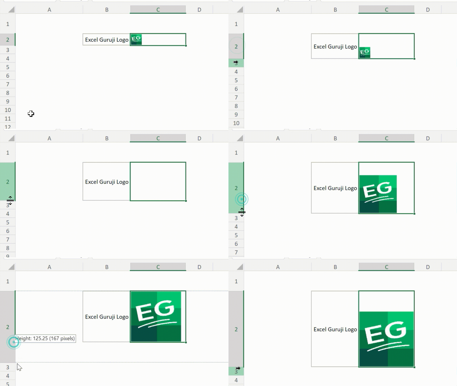
The image will retain its original aspect ratio when you change the cell size.

Image-Function

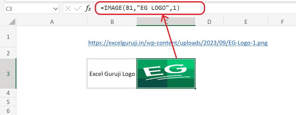
Now, let’s explore the impact by using the other arguments in the Excel IMAGE function’s syntax and observe the resulting effects

Excel IMAGE Function Example 2

Let’s break down this formula: =IMAGE(B1, “EG LOGO”, 1)

  • B1: This is the source argument, 5which contains the URL of the image: “https://excelguruji.in/wp-content/uploads/2023/09/EG-Logo-1.png”. This is the location from which the image will be fetched.
  • “EG LOGO”: This is the alt_text argument, representing alternative text for the image. In this case, it is set to “EG LOGO,” which could be used for accessibility purposes or as a description for the image.
  • 1: The sizing argument, where 1 signifies that the image should fill the entire cell, disregarding its original aspect ratio.
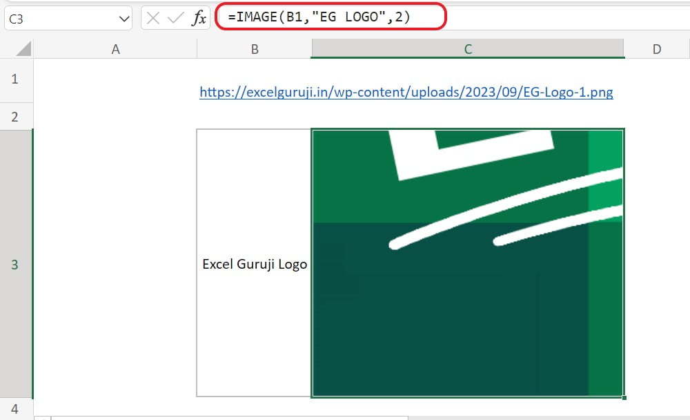
Excel-IMAGE-Function-Example-3

  • 2: When using ‘2’ for sizing, it indicates that the image should maintain its original size, even if it exceeds the cell boundary.

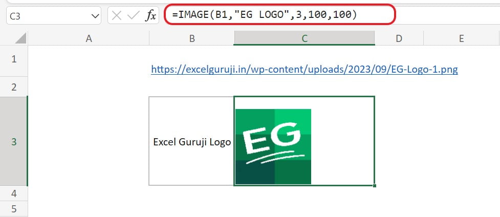
Now, when you set the sizing to ‘3’, you need to specify both the height and width arguments afterward or choose one of them, as demonstrated in the following example.

Excel-IMAGE-Function-Example-4

Even if you alter the size of the cells, the overall image will remain unaffected, which is a positive aspect.

Conclusion

The Excel IMAGE function is a powerful tool for integrating visual elements into your spreadsheets. Experiment with different sizing options, alternative text, and various image types to unleash the full potential of the IMAGE function.

Incorporate visuals into your Excel projects and transform your data into a more dynamic and impactful format.

Frequently Asked Questions (FAQs)

Q1: Can I resize the image using the IMAGE function?

A1: Yes, you can specify the height and width parameters to resize the image.

Q2: Can I use the IMAGE function to insert multiple images in the same worksheet?

A2: Yes, you can use the IMAGE function with different image_ids to insert multiple images in the same worksheet.

Q3: What file formats does the IMAGE function support?

A3: The IMAGE function supports various image file formats, including BMP, JPG/JPEG, PNG, GIF, TIFF, ICO, and WEBP (unsupported on Web and Android).

Q4: How do I handle errors like #VALUE!, #CONNECT!, and #BLOCKED! when using the IMAGE function?

A4: #VALUE! errors may occur for unsupported formats or incorrect parameters. #CONNECT! errors may indicate internet connection issues, and #BLOCKED! errors may be due to security settings. Refer to the documentation for troubleshooting tips.

Other Related Excel Functions

Mastering Excel VLOOKUP Function: A Comprehensive Guide to Enhance Your Data Analysis Skills

Unlocking Data Mastery with Excel HLOOKUP Function: A Comprehensive Guide for Efficient Horizontal Data Lookup

Mastering Excel LOOKUP Function: A Comprehensive Guide to Searching and Retrieving Data in Excel

Join me on Instagram, YouTube and WhatApp Channel for your daily dose of valuable tips and tricks! Catch insightful videos that will enhance your knowledge and skills. Don’t miss out – follow

  1. https://support.microsoft.com/en-au/office/image-function-7e112975-5e52-4f2a-b9da-1d913d51f5d5 ↩︎

Mastering Excel MIN Function: Unveiling Tips and Examples for Efficient Data Analysis

Excel MIN Function

Excel-MIN-Function

When to Use the Excel MIN Function in Excel

The MIN function in Excel comes in handy when you need to find the smallest value in a range of cells. Whether you are working with a dataset, managing financial data, or analyzing performance metrics, the MIN function allows you to quickly identify the minimum value and make data-driven decisions.

What Excel MIN Function Returns

The Excel MIN function returns the smallest value from a given set of numbers or a range of cells.

Syntax of Excel MIN Function

The syntax of the Excel MIN function is as follows:

=MIN(number1, [number2], …)

Input Arguments

Here are the input arguments for the Excel MIN function:

number1: This is the first number, cell reference, or range containing numbers from which you want to find the minimum.

[number2], …: These are optional additional numbers, cell references, or ranges that you can include to find the minimum value among multiple sets of data.

Extra Notes

● Non-numeric values, logical values (TRUE or FALSE), and text representations of numbers are ignored.

● If all the arguments are empty, the function returns a 0.

● If MIN function encounters an error within a range, it will output an error.

● You can input up to 255 arguments.

Examples of the Excel MIN Function

Here are few examples of using the MIN function in Excel:

Example 1: Basic Usage

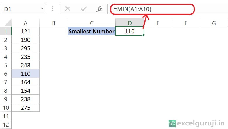
Suppose you have a dataset in cells A1 to A10, and you want to find the smallest value. In cell D1, use the following formula:

Excel-MIN-Function-Example-1

This will return the smallest value in the range.

Example 2: Using Multiple Ranges

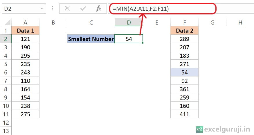
If your dataset is split across different columns, and you want to find the overall minimum, you can use the MIN function with multiple ranges:

Excel-MIN-Function-Example-2

Practice Workbook

Download Free Practice Workbook

Conclusion

In conclusion, the Excel MIN function is a powerful tool for finding the smallest value in a dataset. Whether you are working with financial data, grades, or any numerical information, the MIN function simplifies the process of identifying the minimum value.

Remember, Excel functions are designed to enhance your efficiency and accuracy in data analysis. Practice using the MIN function in different scenarios to become proficient in its application. Start leveraging the MIN function today and take your Excel skills to new heights!

Frequently Asked Questions (FAQs)

Q1: Can the MIN function handle non-numeric values?

A1: No, the MIN function ignores non-numeric values, logical values, and text representations of numbers.

Q2: What happens if all the arguments in the MIN function are empty?

A2: In such cases, the function returns a 0.

Q3: Is there a similar function for finding the minimum based on specific criteria?

A3: Yes, Excel provides the MINIFS function for finding the maximum based on specified conditions.

Q4: Can the MIN function handle more than one range?

A4: Yes, you can use the MIN function with multiple ranges by providing them as separate arguments.

Q5: Are there any limitations to the number of arguments the MIN function can take?

A5: You can input up to 255 arguments in the MIN function.

Other Related Excel Functions

Mastering Excel: Unleashing the Power of the Excel MAX Function for Data Analysis

Unlocking Excel Insights: Mastering the Excel LARGE Function for Advanced Data Analysis and Ranking

Unlocking Data Insights: A Guide to Excel SMALL Function for Precision in Value Extraction

Unlocking the Power of Excel COUNT Function for Accurate Numeric Data Analysis

Mastering Excel COUNTA Function: Counting Non-Empty Cells Made Easy

Join me on Instagram, YouTube and WhatApp Channel for your daily dose of valuable tips and tricks! Catch insightful videos that will enhance your knowledge and skills. Don’t miss out – follow

Unlocking Data Insights: A Guide to Excel SMALL Function for Precision in Value Extraction

Excel SMALL Function

Excel-SMALL-Function

When to Use the Excel SMALL Function in Excel

The SMALL function in Excel comes into play when you need to retrieve the nth smallest value from a set of data. It is particularly useful in scenarios where you are dealing with numerical datasets and want to identify or analyze specific data points based on their magnitude.

What Excel SMALL Function Returns

The Excel SMALL function returns the nth smallest value from a given array or range of cells.

Syntax of Excel SMALL Function

The syntax of the Excel SMALL function is as follows:

=SMALL(array, k)

Input Arguments

Here are the input arguments for the Excel SMALL function:

array: This is the range or array of data from which you want to extract the nth smallest value. It can be a reference to a range of cells or an array of values.

k: The position of the value to retrieve. It must be a positive integer. If k is 1, the function returns the smallest value; if k is 2, it returns the second-smallest, and so on.

Extra Notes

● If k is less than 1 or greater than the number of data points in the array, the function will return a #NUM! error.

● If the array contains non-numeric values, the SMALL function will return a #NUM! error.

● The SMALL function only considers numeric values in the specified array. Empty cells, text values, and boolean values (TRUE and FALSE) are disregarded.

● If all values in the array are non-numeric, the SMALL function returns an error (#NUM!).

Examples of the Excel SMALL Function

Here are few examples of using the SMALL function in Excel:

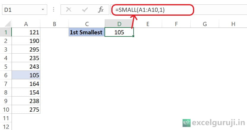
Example 1: Basic Usage

Suppose you have a dataset in cells A1 to A10, and you want to find the smallest value. In cell D1, use the following formula:

Excel-SMALL-Function-Example-1

This will return the smallest value in the range.

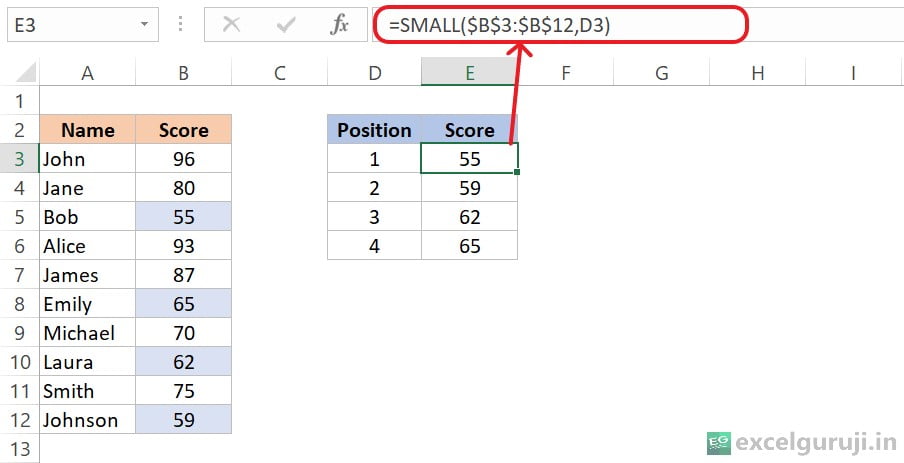
Example 2: Dynamic Use with Cell Reference

Suppose you have the value of ‘k’ in cells D3 to D6, and you want to dynamically change the position. Use the following formula:

Excel-SMALL-Function-Example-2

let’s break down the formula: =SMALL($B$3:$B$12,D3)

  • $B$3:$B$12: This part refers to a specific range of cells in column B, from cell B3 to B12. The dollar signs ($) before the column and row references mean that these references are absolute, which implies that they won’t change when you copy the formula to other cells.
  • D3: This is the second argument or parameter for the SMALL function. It represents the position of the smallest value you want to find. In this case, it is in cell D3. If D3 contains the number 1, it will find the smallest value; if it contains 2, it will find the second-smallest, and so on.

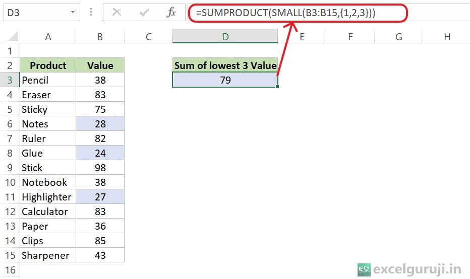
Example 3: Summing the Values with SUMPRODUCT and SMALL Functions

Imagine you manage an office supplies store, and you have a dataset containing information about various products and their respective values. Your goal is to sum the lowest 3 values from the array. To achieve this, you use the Excel SUMPRODUCT function in conjunction with the SMALL function.

Excel-SMALL-Function-Example-3

let’s break down the formula: =SUMPRODUCT(SMALL(B3:B15, {1,2,3}))

  • B3:B15: This is the range of values in column B from cell B3 to B15.
  • SMALL(B3:B15, {1,2,3}): The SMALL function is finding the 1st, 2nd, and 3rd lowest values in the specified range. The curly braces “{1,2,3}” are used to create an array that tells the SMALL function which positions to consider. It is saying, “Find the 1st, 2nd, and 3rd lowest values”,
  • SUMPRODUCT(SMALL(B3:B15, {1,2,3})): The SUMPRODUCT function then takes these three values found by the SMALL function and adds them together.

So, the array “{1,2,3}” serves as a set of positions (1st, 2nd, and 3rd) to be considered by the SMALL function, allowing you to customize which smallest values you want to include in the sum.

Practice Workbook

Download Free Practice Workbook

Conclusion

In conclusion, the Excel SMALL function is a powerful tool for extracting specific values based on their position in a dataset. Whether you are working with financial data, analyzing exam results, or managing project deadlines, the Excel SMALL function can help you identify and analyze the relevant data points.

As with any Excel function, it is important to understand the syntax and input requirements. Practice using the Excel SMALL function in different scenarios to enhance your Excel skills and improve your data analysis capabilities.

Frequently Asked Questions (FAQs)

Q1: Can the SMALL function be used to find the largest values in a dataset?

A1: No, the SMALL function is specifically designed to find the smallest values. To find the largest values, you should use the LARGE function.

Q2: What happens if the specified rank (k) is greater than the number of data points in the array?

A2: In such cases, the SMALL function returns a #NUM! error. Make sure that the rank is within the range of available data points.

Q3: Can the SMALL function handle non-numeric values in the array?

A3: No, the SMALL function is designed for numerical data. If the array contains non-numeric values, the function returns a #NUM! error.

Q4: Can I use a cell reference for the ‘k’ argument?

A4: Yes, you can use a cell reference to dynamically change the position of the value to retrieve.

Q5: Are there any restrictions on the type of values in the array?

A5: The array should contain numeric values; otherwise, the function will return the #NUM! error.

Other Related Excel Functions

Unlocking the Power of Excel COUNT Function for Accurate Numeric Data Analysis

Mastering Excel COUNTA Function: Counting Non-Empty Cells Made Easy

Excel COUNTBLANK Function: How to Count Empty Cells in Excel

Join me on Instagram, YouTube and WhatApp Channel for your daily dose of valuable tips and tricks! Catch insightful videos that will enhance your knowledge and skills. Don’t miss out – follow me now!
Unlocking Excel Insights: Mastering the Excel LARGE Function for Advanced Data Analysis and Ranking

Excel LARGE Function

Excel-LARGE-Function

When to Use the Excel LARGE Function in Excel

The Excel LARGE function is a powerful tool when you need to extract the k-th largest value from a set of values in a range. It is particularly useful for analyzing datasets, identifying top performers, or ranking numerical data.

What Excel LARGE Function Returns

The Excel LARGE function returns the k-th largest value from a given range. The ‘k’ value is specified by the user and determines which largest value to extract from the dataset.

Syntax of Excel LARGE Function

The syntax of the Excel LARGE function is as follows:

=LARGE(array, k)

Input Arguments

Here are the input arguments for the Excel LARGE function:

array: The range of cells or an array containing the numeric values from which you want to extract the k-th largest value.

k: The position of the value to retrieve. It must be a positive integer. If k is 1, the function returns the largest value; if k is 2, it returns the second-largest, and so on.

Extra Notes

● If the specified ‘k’ is greater than the number of values in the array, the function returns the #NUM! error.
● If ‘k’ is not a positive integer, the function returns the #NUM! error.

● The LARGE function only considers numeric values in the specified array. Empty cells, text values, and boolean values (TRUE and FALSE) are disregarded.

● If all values in the array are non-numeric, the LARGE function returns an error (#NUM!).

Examples of the Excel LARGE Function

Here are few examples of using the LARGE function in Excel:

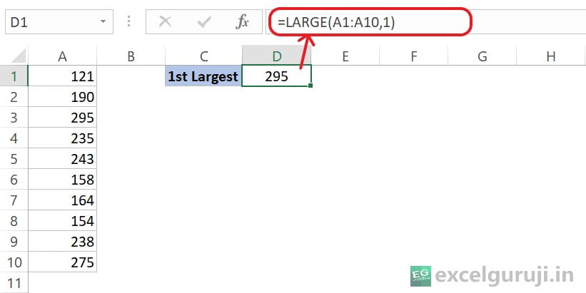
Example 1: Basic Usage

Suppose you have a dataset in cells A1 to A10, and you want to find the largest value. In cell D1, use the following formula:

Excel-LARGE-Function-Example-1

This will return the largest value in the range.

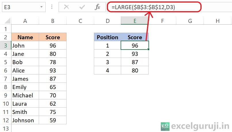
Example 2: Dynamic Use with Cell Reference

Suppose you have the value of ‘k’ in cells D3 to D6, and you want to dynamically change the position. Use the following formula:

Excel LARGE Function Example 2

let’s break down the formula: =LARGE($B$3:$B$12,D3)

  • $B$3:$B$12: This part refers to a specific range of cells in column B, from cell B3 to B12. The dollar signs ($) before the column and row references mean that these references are absolute, which implies that they won’t change when you copy the formula to other cells.
  • D3: This is the second argument or parameter for the LARGE function. It represents the position of the largest value you want to find. In this case, it is in cell D3. If D3 contains the number 1, it will find the largest value; if it contains 2, it will find the second-largest, and so on.

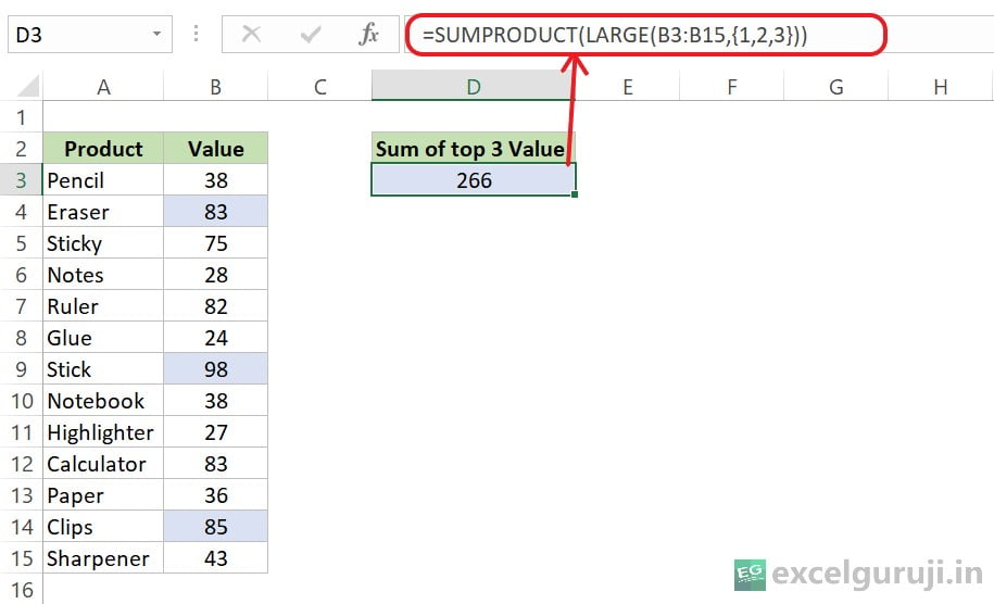
Example 3: Summing Top Values with SUMPRODUCT and LARGE Functions

Imagine you manage an office supplies store, and you have a dataset containing information about various products and their respective values. Your goal is to sum the top 3 values from the given range. To achieve this, you use the Excel SUMPRODUCT function in conjunction with the LARGE function.

Excel-LARGE-Function-Example-3

let’s break down the formula: =SUMPRODUCT(LARGE(B3:B15, {1,2,3}))

  • B3:B15: This is the range of values in column B from cell B3 to B15.
  • LARGE(B3:B15, {1,2,3}): The LARGE function is finding the 1st, 2nd, and 3rd largest values in the specified range. The curly braces “{1,2,3}” are used to create an array that tells the LARGE function which positions to consider. It is saying, “Find the 1st, 2nd, and 3rd largest values”,
  • SUMPRODUCT(LARGE(B3:B15, {1,2,3})): The SUMPRODUCT function then takes these three values found by the LARGE function and adds them together.

So, the array “{1,2,3}” serves as a set of positions (1st, 2nd, and 3rd) to be considered by the LARGE function, allowing you to customize which largest values you want to include in the sum.

Practice Workbook

Download Free Practice Workbook

Conclusion

In conclusion, the Excel LARGE function is an invaluable tool for extracting specific values based on their position in a dataset. Whether you are analyzing financial data, ranking performance, or conducting statistical analysis, the LARGE function can simplify your tasks and provide meaningful insights.

Remember, exploring different applications of the LARGE function in real-world scenarios will enhance your proficiency in Excel. Practice and experimentation are key to mastering Excel functions. Start using the LARGE function today and take your Excel skills to the next level!

Frequently Asked Questions (FAQs)

Q1: Can the LARGE function be used to find the smallest value?

A1: No, the LARGE function is designed specifically to find the k-th largest value.

Q2: Is the LARGE function sensitive to the order of values in the array?

A2: No, the LARGE function looks for the k-th largest value regardless of the order of values in the array.

Q3: What happens if ‘k’ is greater than the number of values in the array?

A3: In such cases, the function returns the #NUM! error.

Q4: Can I use a cell reference for the ‘k’ argument?

A4: Yes, you can use a cell reference to dynamically change the position of the value to retrieve.

Q5: Are there any restrictions on the type of values in the array?

A5: The array should contain numeric values; otherwise, the function will return the #NUM! error.

Other Related Excel Functions

Unlocking the Power of Excel COUNT Function for Accurate Numeric Data Analysis

Mastering Excel COUNTA Function: Counting Non-Empty Cells Made Easy

Excel COUNTBLANK Function: How to Count Empty Cells in Excel

Join me on Instagram, YouTube and WhatApp Channel for your daily dose of valuable tips and tricks! Catch insightful videos that will enhance your knowledge and skills. Don’t miss out – follow me now!