Mastering Excel: 10 Quick Techniques to Sum

In the world of spreadsheets, Excel is the top choice for analyzing, reporting, and doing calculations. Whether you are experienced with Excel or just starting out, learning how to add up data can really make your work easier and faster.

In this complete guide, we will look at 10 important tips, to help you sum up data in Excel in a better way.

If you prefer watching videos over reading the blog, you can view this video.

10 Methods to Find Sum in Excel

And if you are interested in reading the blog, please continue reading.

Add Up Numbers Yourself in Excel

Manually summing data in Excel is the most basic yet fundamental method of calculating totals. This approach involves directly inputting formulas into cells to perform arithmetic operations.

Here is a detailed breakdown of how to utilize this technique effectively:

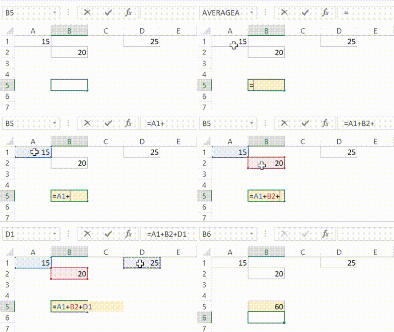
1. Select the Destination Cell: Begin by selecting the cell where you want the sum to appear.

2. Input the Formula: To initiate manual summation, start typing the equal sign (=) into the selected cell.

3. Reference the Cells to Sum: After typing the equal sign, click on the first cell you want to include in the sum. For instance, if you want to sum the values in cells A1, B2, and D1, click on cell A1 after typing the equal sign.

4. Enter the Operator: Following the cell reference, input the operator that corresponds to the arithmetic operation you wish to perform. For addition, use the plus sign (+).

5. Repeat for Additional Cells: After entering the operator, click on the next cell you want to include in the sum. Continue this process until you have referenced all the cells you want to sum.

6. Complete the Formula: Once you have referenced all the cells, press Enter to complete the formula. Excel will calculate the sum of the selected cells and display the result in the destination cell.
Add Up Numbers Yourself

Manual Summation offers simplicity and immediate results but is prone to errors and lacks automation, remaining a fundamental skill in Excel.

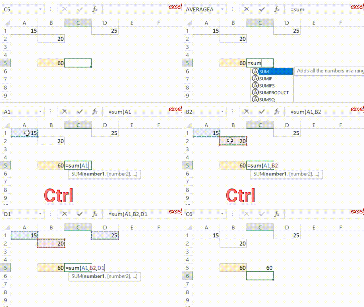
In this case, you can also use the SUM function, eliminating the need for adding plus signs. Simply open the bracket and select the desired cells while holding down the CTRL key.
Add Up Numbers Yourself2

You can use this method when you need to calculate the total of two to three non-contiguous cells.

Quick Way with Shortcut Key (Alt+=)

Utilizing keyboard shortcuts in Excel can significantly enhance your workflow by providing quick access to frequently used functions. Among these shortcuts, the combination of the Alt key with the equals sign (=) stands out as an efficient way to perform data summation.

Here is a detailed explanation of how to leverage this shortcut effectively:

1. Select the Range: Either Choose the range of cells you want to sum, or make sure the last cell of your range is selected.

2. Press Alt+=: Once you have selected the range, simply press and hold the Alt key on your keyboard and then press the equals sign (=). This keyboard shortcut tells Excel to auto-sum the selected range and place the total in the active cell.
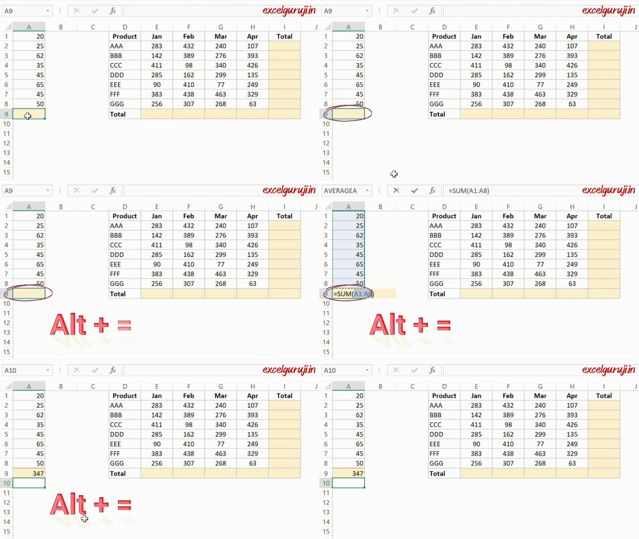
Quick Way with Shortcut Key1

The advantage of shortcut keys is that you can perform multiple sums at once, as demonstrated in the example below.
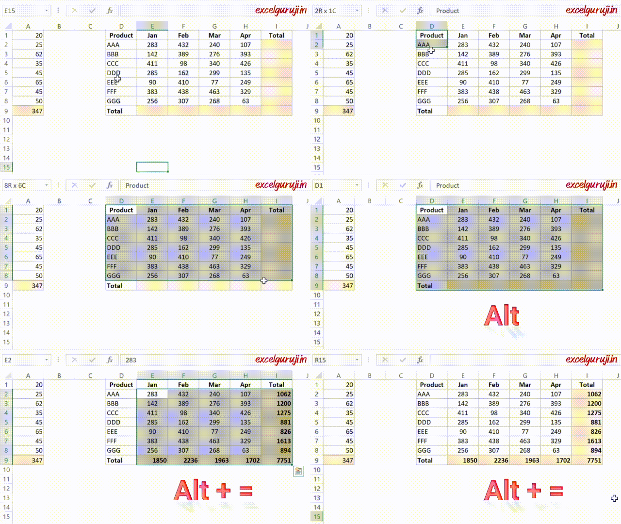
Quick Way with Shortcut Key2

Shortcut Key Summation offers speed and ease of use, enabling quick calculations across various cell ranges. However, it is limited to basic sums and requires precise selection, though additional tips enhance its efficiency in Excel tasks.

Using SUM Function in Excel the Easy Way

Excel’s built-in SUM function is a powerful tool for summing data in spreadsheets. While it is commonly used, understanding how to use it manually can provide greater control and flexibility over your calculations.

Now, you may think, ‘We know the shortcut keys, so why should we use the function manually?’

We will use the sum function manually because if there is a blank cell within the range, automatic selection extends to the fill cells, as shown in the figure below.
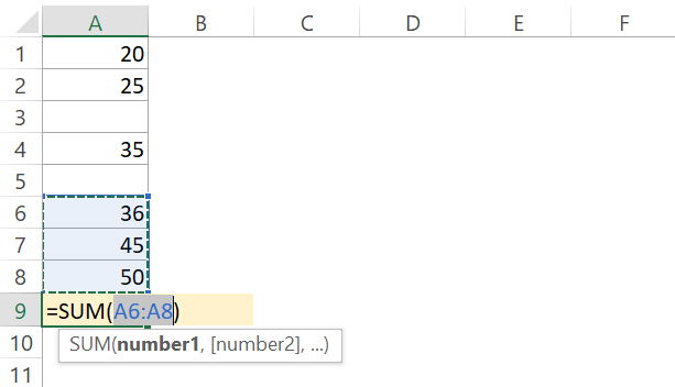
10 Quick Techniques to Sum Tips3

Here is a detailed guide on leveraging the SUM function effectively:

1. Select the Destination Cell: Begin by selecting the cell where you want the sum to appear.

2. Input the Formula: Type the equal sign (=) into the selected cell to start entering a formula. Then, type “SUM(” to initiate the SUM function.

3. Specify the Range: After typing “SUM(“, specify the range of cells you want to sum. You can do this by typing cell references (e.g., A1:A8) or clicking and dragging to select the range visually. Excel will automatically insert the range into the formula.

4. Close the Function: Once you have specified the range, close the SUM function by typing a closing parenthesis ). Ensure that there are no extra or missing parentheses to avoid errors.
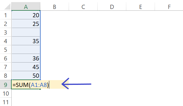
10 Quick Techniques to Sum Tips4

5. Press Enter: After completing the formula, press Enter to calculate the sum. Excel will display the total sum in the selected cell.

Fixing Mistakes with Aggregate Function

When you perform a sum in Excel and encounter errors within your range, those errors will also be reflected in the result.
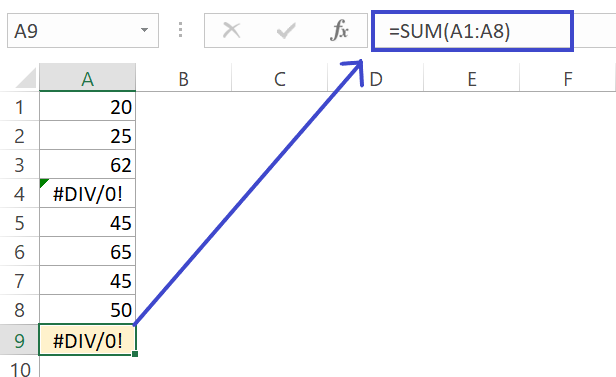
10 Quick Techniques to Sum Tips5

In Excel, the AGGREGATE function is a versatile tool that offers advanced capabilities for data analysis and manipulation, including error handling.

Understanding how to use the AGGREGATE function can enhance your ability to perform accurate summations, even in the presence of errors or hidden data.

Here is a detailed guide on leveraging the AGGREGATE function effectively:

1. Select the Destination Cell: Begin by selecting the cell where you want the sum to appear. This is where you will input the AGGREGATE function.

2. Input the Formula: Type the equal sign (=) into the selected cell to start entering a formula. Then, type “AGGREGATE(” to initiate the AGGREGATE function. The AGGREGATE function has the following syntax: =AGGREGATE(function_num, options, [array], [k]).

3. Specify the Function Number and Options: Enter the desired function number (e.g., 9 for SUM) and the desired options (e.g., 6 for ignoring errors) separated by commas.

4. Specify the Data Range: After specifying the function and options, provide the range of cells or array containing the data you want to sum.

5. Press Enter: After completing the formula, press Enter to calculate the sum. Excel will display the total sum in the selected cell, taking into account the specified function, options, and data range.
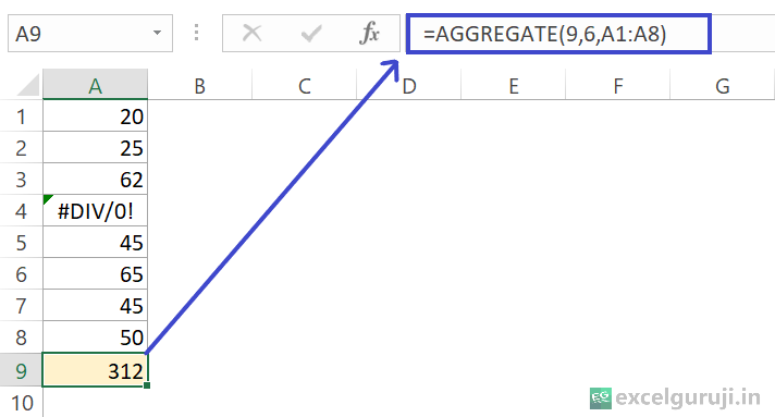
10 Quick Techniques to Sum Tips6

Fast Summary with Quick Analysis Tool

If you are using Excel 2013 or a newer version, Excel’s Quick Analysis tool is a fantastic feature that offers an easy way to do different data analysis tasks like adding up data, making charts, and formatting.

Knowing how to use this tool well can make your work easier and help you get more done.

Here is a thorough guide on how to use the Quick Analysis tool for adding up data:

1. Select the Data Range: Begin by selecting the range of cells that you want to analyze and sum.

2. Access the Quick Analysis Tool: Once you have selected the data range, a small icon (a square with a lightening bolt) will appear in the bottom-right corner of the selected range. Alternatively, you can right-click on the selected range to bring up a context menu, then choose “Quick Analysis” from the options provided.

3. Explore Summation Options: Clicking on the Quick Analysis icon opens a menu with various analysis options. To perform summation, click on the “Totals” tab in the Quick Analysis menu.

4. Select Summation Option: In the Totals tab, you’ll find several summation options, including Sum, Average, Count, and more. Click on the “Sum” option to instantly calculate the sum of the selected data range.

5. Review and Confirm: After selecting the Sum option, Excel will display the calculated sum in the preview window. Take a moment to review the result and ensure that it matches your expectations.
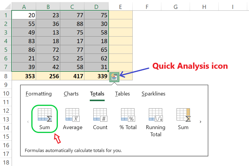
10 Quick Techniques to Sum Tips7

The Quick Analysis tool in Excel provides speedy and intuitive summation capabilities with visual previews, enhancing efficiency and accessibility for users of all levels.

Additionally, it offers various other analysis options for comprehensive data exploration and can be combined with advanced Excel features for more intricate analysis tasks.

Making Totals with Filtered Lists

When working with filtered lists in Excel, maintaining accurate totals can be challenging due to the dynamic nature of the data.

The SUBTOTAL function addresses this challenge by automatically adjusting totals based on applied filters, providing accurate summaries even in filtered data sets.

Here is a detailed guide on how to use the SUBTOTAL function effectively:

1. Understanding the SUBTOTAL Function: The SUBTOTAL function performs calculations (such as summation) on a range of cells, taking into account only the visible cells and ignoring any hidden or filtered-out cells.

2. Select the Destination Cell: Begin by selecting the cell where you want the subtotal to appear. This is where you’ll input the SUBTOTAL function.

3. Input the Formula: Type the equal sign (=) into the selected cell to start entering a formula. Then, type “SUBTOTAL(” to initiate the SUBTOTAL function. The SUBTOTAL function has the following syntax: SUBTOTAL(function_num, ref1, [ref2], …).

4. Specify the Function Number: Enter the desired function number (e.g., 109 for SUM) as the first argument of the SUBTOTAL function. This determines the type of calculation to perform.

5. Specify the Data Range: After specifying the function number, provide the range of cells containing the data you want to include in the subtotal calculation (close the SUBTOTAL function by typing a closing parenthesis).

6. Press Enter: After completing the formula, press Enter to calculate the subtotal. Excel will display the total sum in the selected cell, adjusting the calculation based on any applied filters.
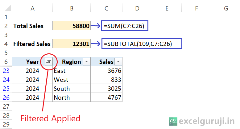
10 Quick Techniques to Sum Tips8

The SUBTOTAL function in Excel ensures accurate totals by dynamically adjusting calculations based on applied filters, offering versatility for various functions.

Experiment with filters and nested formulas to optimize data analysis and reporting, ensuring reliability and integrity in your spreadsheets.

Clearer Adding: Using Table Names

Using table names in Excel formulas, including the SUM function, enhances clarity, ease of use, and maintainability, especially in complex spreadsheets.

Tables provide a structured way to organize and reference data, and incorporating table names into formulas improves formula readability and simplifies spreadsheet navigation.

Suppose we have the following data
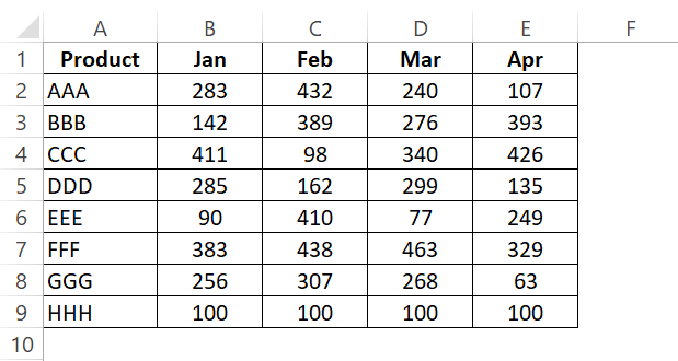
10 Quick Techniques to Sum TipsTable

Here is a detailed guide on how to use table names effectively in the SUM function:

1. Create a Table: To create a table, select the range of cells containing your data, then go to the “Insert” tab on the Excel ribbon and click on “Table” (Shortcut Key – Ctrl + T). Excel will automatically detect the range and convert it into a table format.

2. Understanding Table References: When you create a table, Excel automatically assigns a structured reference to the table. This structured reference consists of the table name followed by column names enclosed in square brackets (e.g., TableName[ColumnName]). These structured references make it easy to reference specific columns within the table.

3. Using Table Names in SUM Function: To use a table name in the SUM function, simply type the table name followed by the column name inside square brackets. For example, if you have a table named “Table1” with a column named “Feb”, you can use the following formula to sum the Feb
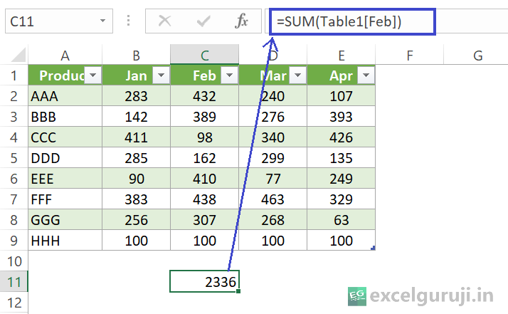
10 Quick Techniques to Sum TipsTable1

Using table names in formulas like SUM improves spreadsheet readability and maintenance by automatically adjusting to table changes, ensuring accurate calculations and reducing manual updates.

Consistent naming conventions and structured references further enhance clarity and efficiency in data analysis tasks.

Simple Adding: Using Named Ranges

Named ranges offer a powerful way to organize and manage data in Excel.

By assigning meaningful names to ranges of cells and incorporating them into SUM functions, you can improve formula readability, simplify spreadsheet navigation, and streamline your data analysis workflows.

Here is a detailed guide on how to use named ranges effectively in the SUM function:

1. Define Named Ranges: Before using named ranges in formulas, you need to define them in Excel. To define a named range, select the range of cells you want to name, then go to the “Formulas” tab on the Excel ribbon and click on “Create from Selection”.

10 Quick Techniques to Sum TipsName Range

Click the checkboxes for Top row and Left column in the dialog box that appears, then click OK.
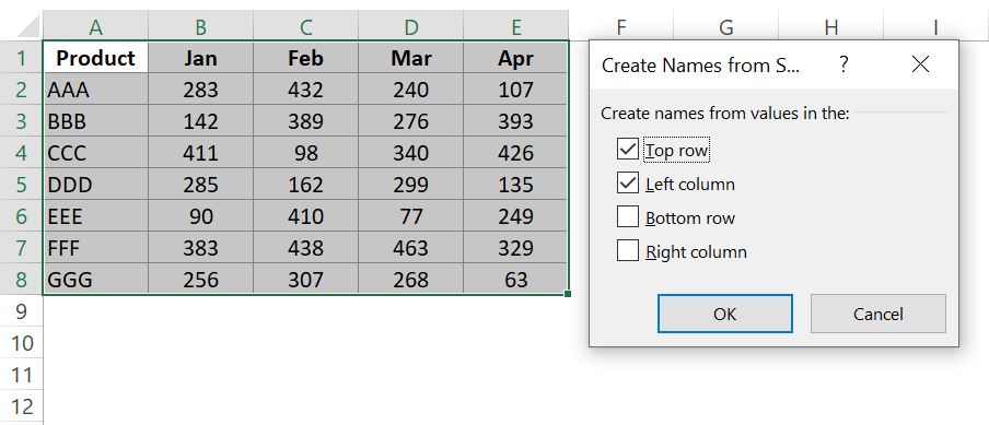
10 Quick Techniques to Sum TipsName Range1

2. Understanding Named Range References: Once you have defined a named range, you can reference it in formulas using the name you assigned. Named range references are absolute and do not change when you copy or move formulas containing them.

This makes named ranges particularly useful for referencing data that remains constant or needs to be referenced across multiple worksheets.

3. Using Named Ranges in SUM Function: To use a named range in the SUM function, simply type the name of the range instead of specifying cell references. For example, if you have a named range called “Mar” that refers to cells D2:D8, you can use the following formula to sum the values in the named range:
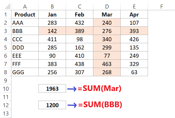
10 Quick Techniques to Sum TipsName Range2

Leveraging SUMIF & SUMIFS for Conditional Summing

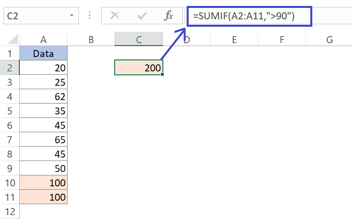
The SUMIF function in Excel adds the cells specified by a given condition or criteria. It is useful for summing values in a range that meet specific criteria.

On the other hand, the SUMIFS function in Excel adds the cells specified by multiple conditions or criteria. It is an extension of the SUMIF function and allows for more complex conditional summation.

Here is how to use it:
10 Quick Techniques to Sum TipsSUMIF1

In the example, we used SUMIF to add numbers above 90 in our range. We found only two cells with values over 90, both being 100. If you need multiple conditions, try SUMIFS.

Harnessing the Power of SUMPRODUCT for Advanced Calculations

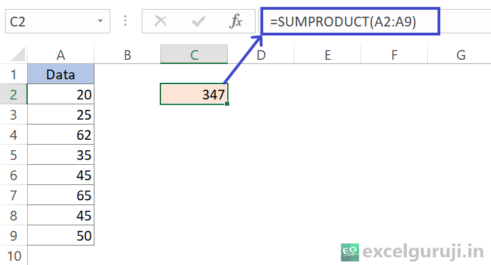
The SUMPRODUCT function in Excel calculates the sum of products by multiplying corresponding arrays or ranges.

However, it is important to note that if you only have one range to sum, you can still utilize the SUMPRODUCT function.

Conversely, if you have multiple ranges, you cannot employ the SUMPRODUCT function.

Here’s how to use it:
10 Quick Techniques to Sum TipsSUMPRODUCT

Easy Analysis with Pivot Tables

Pivot Tables are indispensable tools for dynamic data analysis and summarization in Excel. They offer a powerful way to analyze large datasets, generate insightful summaries, perform calculations, and visualize trends with ease.

Understanding how to use Pivot Tables effectively can revolutionize your approach to data summation and analysis.

Here is a detailed guide on leveraging Pivot Tables for data summation:

1. Creating a Pivot Table: To create a Pivot Table, follow these steps:

• Select the range of data you want to analyze.
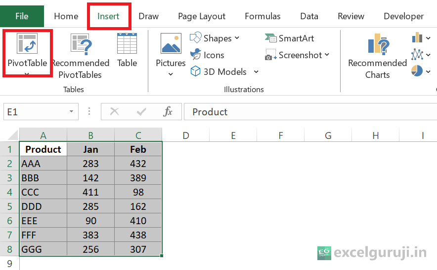
• Go to the “Insert” tab on the Excel ribbon and click on “Pivot Table.”
10 Quick Techniques to Sum TipsPivot Table

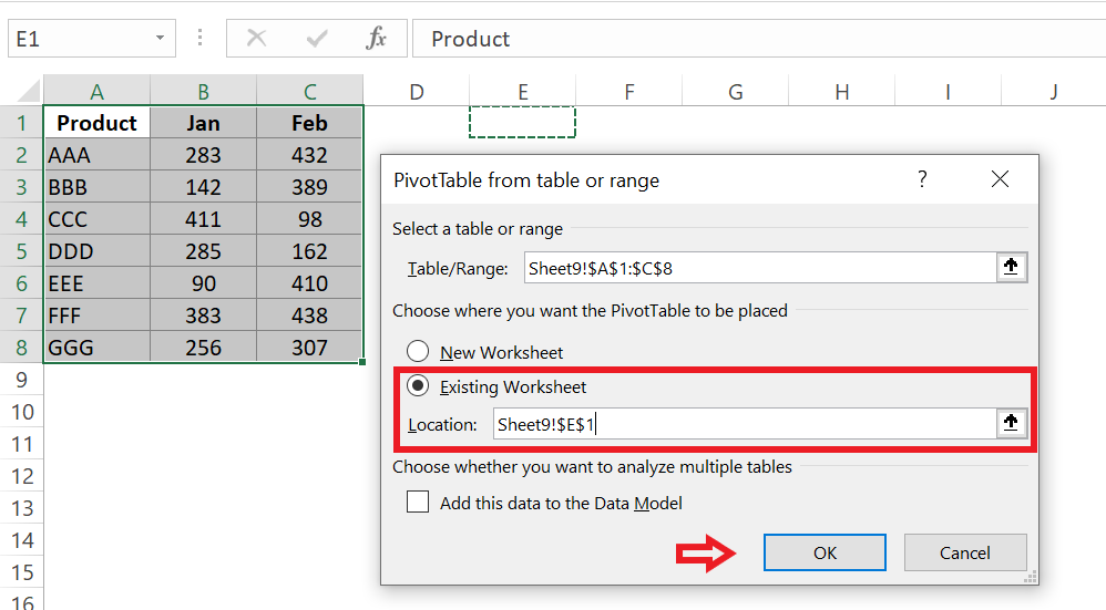
• In the Create PivotTable dialog box, specify where you want to place the Pivot Table (e.g., Existing Worksheet) and click “OK.”
10 Quick Techniques to Sum TipsPivot Table1

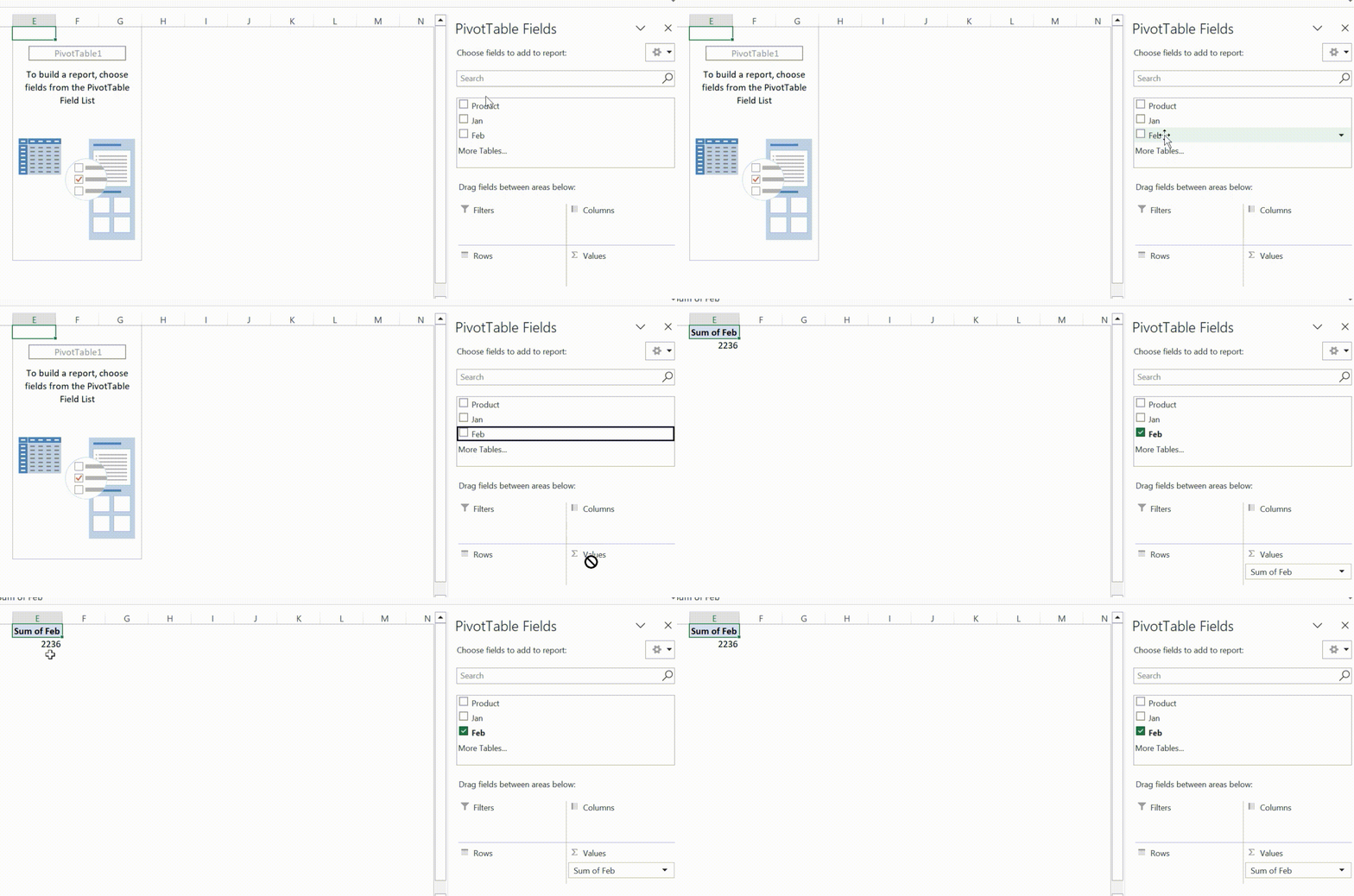
2. Configuring the Pivot Table Fields: After creating the Pivot Table, Excel will display the PivotTable Field List pane. This pane contains a list of all the fields (columns) from your data range.

To perform summation, drag the field containing the values you wish to sum into the “Values” area. For instance, if you want the total of the Feb field, you drag it and place it in the value area.

Excel will then automatically sum the values and display the total.
10 Quick Techniques to Sum TipsPivot Table1

Pivot Tables help you understand big sets of data quickly and in different ways. They can show you trends and let you look at details easily.

Trying out different Pivot Table features can make your data analysis better, and don’t forget to update your data if it changes.

Making Data Better with Power Query

Power Query, a feature available in Excel (as well as other Microsoft products like Power BI), empowers users to transform, clean, and merge data from various sources seamlessly.

Here is a detailed guide on leveraging Power Query for data summation:

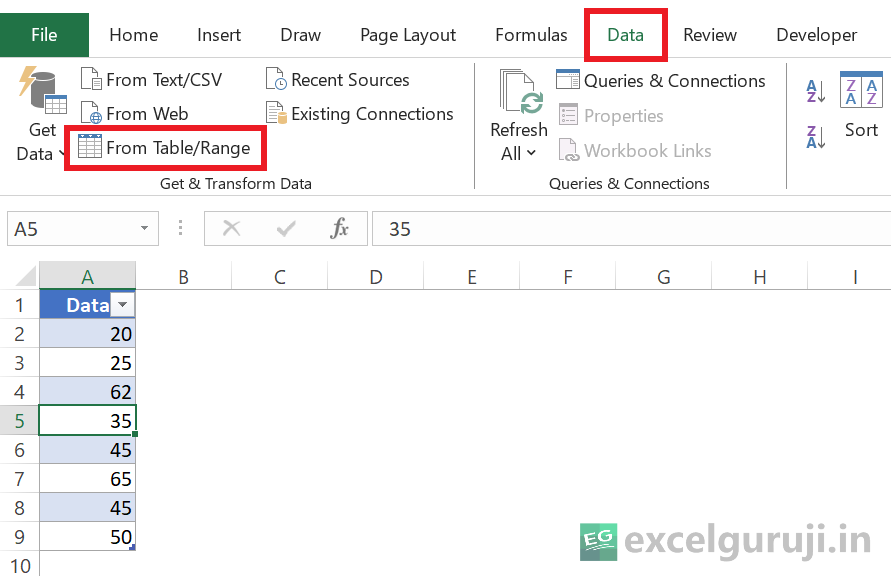
1. Select the data range you want to work with or click on any cell within your dataset.

2. Go to the “Data” tab on the Excel ribbon and click on “Get Data” or “From Table/Range” (depending on your Excel version).
10 Quick Techniques to Sum TipsPower Query1

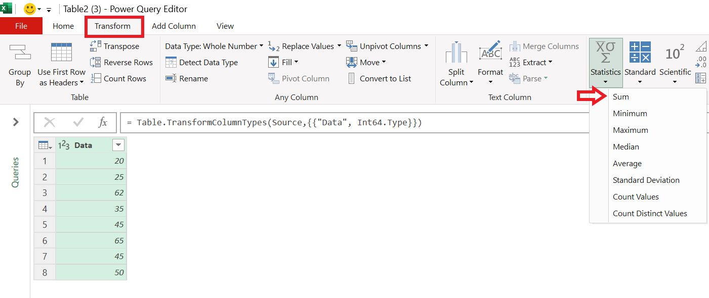
3. While in the Power Query Editor, navigate to the Transform menu and choose “SUM” from the statistics options.
10 Quick Techniques to Sum TipsPower Query2

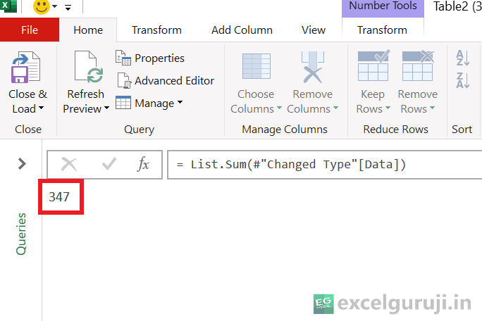
4. Power Query will produce the aggregated results.
10 Quick Techniques to Sum TipsPower Query3

5. After completing your data transformations and aggregations in Power Query, you can load the transformed data back into Excel.

6. Click on the “Close & Load to” button on the File Menu.

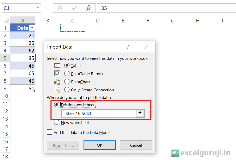
7. Choose whether you want to load the data to a new worksheet, an existing worksheet.
10 Quick Techniques to Sum TipsPower Query5

8. Click “OK” to import the transformed data into Excel.

One of the key benefits of using Power Query is the ability to refresh your data with a single click. If your original data source changes or updates, you can simply click the “Refresh” button in Excel to update your Power Query transformations and calculations accordingly.

Sum Directly from Status Bar

In Excel, you can easily sum a range of cells directly from the status bar.

Here is how you can do it:

Select the range of cells that you want to sum.

Look at the bottom-right corner of the Excel window, where you will find the status bar.

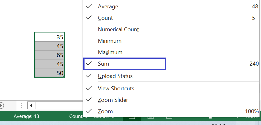
By default, the status bar shows the sum of the selected cells. If you selected a range of numbers, you should see the sum displayed in the status bar. If the sum is not displayed in the status bar, you might need to right-click on the status bar and ensure that the “Sum” option is checked.
10 Quick Techniques to Sum TipsStatus Bar

Once the “Sum” option is enabled, Excel will display the sum of the selected cells in the status bar whenever you have a range of cells selected.

To copy this total, left-click on the total displayed in the status bar. Then, select the cell where you want the total to appear and press Ctrl + V to paste it.

10 Quick Techniques to Sum TipsStatus Bar

We were tasked with summing up with 10 methods, but in the process, we ended up with 13! I hope you have enjoyed learning all of these helpful Excel tips.

Below is the link to download the practice Excel file for free. Feel free to explore and practice all the tips yourself:

Download Free Excel File For Practice

Happy Excel-ing!

How to Create a Drop Down List in Excel

How to Create a Drop Down List in Excel

Drop down lists are like magic boxes in Excel – they offer pre-defined choices, making data entry a breeze and reducing errors. This guide, explains everything you need to know about drop down lists.

Video Tutorial – How to create a drop down list in Excel

How to create a drop down list in Excel

What are Drop Down Lists in Excel?

Imagine a cell in your spreadsheet. Instead of typing things in every time, you want users to choose from a specific set of options. That is where drop down lists come in! They display a small arrow, and clicking it reveals a list of choices users can select.

Benefits:

1. Faster and easier data entry: No more typing the same things repeatedly!

2. Reduced errors: Users can only choose from pre-defined options, minimizing typos and inconsistencies.

3. Improved data consistency: Ensures everyone uses the same terms and values.

How to Create Drop Down List in Excel?

There are several ways to create drop down lists, depending on how you have your data organized:

1. Entering choices manually

2. Using range of cells

3. Using named ranges

4. Using formula (Dynamic drop down list)

By Entering Choices Manually

For example, if you wish to create a drop down list within a cell with three options, Yes and No, here is how you can input manually them directly into the data validation source field.

1. Choose the cell where you want the drop down list. It can be a single cell, a range of cells, a whole column, or non-continuous cells. (To select non-continuous cells, press the Ctrl key and then select each desired cell.)

2. Go to the “Data” tab on the top ribbon.

3. Click the “Data Validation” button in the “Data Tools” ribbon.

How to Create a Drop Down List in Excel Manually Choice 1

4. In the Data Validation window, choose the “Settings” tab.

5. From the Allow drop down menu, select “List”.

6. Type your list of choices separated by commas (with or without spaces), like “Yes, No

7. Click “OK” to save and activate the drop down list.

How to Create a Drop Down List in Excel Manually Choice 2

Note: Ensure that the “In-cell drop down” option is checked (which is the default setting); otherwise, the drop down arrow will not appear next to the cell.

How-to-Create-a-Drop-Down-List-in-Excel-Manual.gif

By Using Range of Cells

If you have a predefined list of options in a separate range of cells, you can reference that range to create your drop down list.

Follow the same steps as above, but instead of manually entering the options, select the range containing the data you want to use.

1. Make a separate list of options somewhere on your sheet.

2. Choose the cell where you want the drop down list.

3. Go to the “Data” tab on the top ribbon.

4. Click the “Data Validation” button in the “Data Tools” ribbon.

How to Create a Drop Down List in Excel Select Range 1

5. In the Data Validation window, choose the “Settings” tab.

6. From the Allow drop down menu, select “List”.

7. Enter the cell range of your list in the “Source” box.

8. Click “OK” to save and activate the drop down list.

How to Create a Drop Down List in Excel Select Range 2

By Using Name Range

Named ranges provide a convenient way to refer to a specific range of cells by a custom name.

Define a named range for your list of options, and then use that name when setting up data validation to create your drop down list.

1. Select a cell or group of cells you wish to assign a name to.

2. Enter a name in the Name Box and press Enter key

For example, let’s name the range ‘vegetables’.

How to Create a Drop Down List in Excel Name Range 1

3. Choose the cell where you want the drop down list.

4. Go to the “Data” tab on the top ribbon.

5. Click the “Data Validation” button in the “Data Tools” ribbon.

How to Create a Drop Down List in Excel Name Range 2

6. In the Data Validation window, choose the “Settings” tab.

7. From the Allow drop down menu, select “List”.

8. Enter the name range as =vegetables in the “Source” box.

9. Click “OK” to save and activate the drop down list.

How to Create a Drop Down List in Excel Name Range 3

Tips💡: When you insert multiple drop downs in different sheets, using named ranges makes them easier to identify and manage

Create Dynamic Drop Down List

Static drop down lists are useful, but sometimes you need them to adjust dynamically based on changes in the source data. This is where dynamic drop down lists come into play.

By leveraging Excel’s functions like OFFSET, you can create drop down lists that automatically update as your data changes.

Below is the method for creating a dynamic drop down:

1. Choose the cell where you want the drop down list. It can be a single cell, a range of cells, a whole column, or non-continuous cells. (To select non-continuous cells, press the Ctrl key and then select each desired cell.)

2. Go to the “Data” tab on the top ribbon.

3. Click the “Data Validation” button in the “Data Tools” ribbon.

How to Create a Drop Down List in Excel Dynamic 1

4. In the Data Validation window, choose the “Settings” tab.

5. From the Allow drop down menu, select “List”.

6. Use the following formula in the source field: =OFFSET($A$2:$A$20,0,0,COUNTA($A$2:$A$20))

7. Click “OK” to save and activate the drop down list.

How to Create a Drop Down List in Excel Dynamic 2

Benefits of this formula:

The formula automatically adjusts the size of the drop down list based on the number of entries in your data.

If you add or remove items in A2:A20, the drop down list will update accordingly.

How to Create a Drop Down List in Excel Dynamic 3

Here is a breakdown of how this formula works: =OFFSET($A$2:$A$20,0,0,COUNTA($A$2:$A$20))

The syntax of the Excel OFFSET function is: =OFFSET(reference, rows, cols, [height], [width])

The syntax of the Excel COUNTA function is: =COUNTA(value1, [value2], …)

OFFSET: This function returns a reference to a range that is offset from a starting cell or range of cells by a specified number of rows and columns. It is commonly used for dynamic range references.

$A$2:$A$20: This is the starting range. In this case, it is the range of cells from A2 to A20. This is the range from which the drop down list values will be derived. The dollar signs ($) make the reference absolute, meaning it won’t change if you copy the formula to another cell.

0, 0: These are the number of rows and columns by which the range specified in the first argument (A2:A20) will be offset. Here, both are set to 0, meaning there is no offset. This indicates that the drop down list will start from the first cell of the specified range.

COUNTA($A$2:$A$20): This function counts the number of non-empty cells in the range A2:A20. It is used here to dynamically determine the height of the range for the drop down list. This ensures that the drop down list only includes non-empty cells within the specified range.

Note: To make sure it works, there shouldn’t be any empty cell between the filled cells.

Create a Dependable Drop Down List

A dependable drop down list is where the options in a second drop down are adjusted based on the selection made in the first.

Below is the example of dependable drop down list

How to Create a Drop Down List in Excel Dependable 1

In the example above, the options in ‘Drop Down 2’ change based on what you pick in ‘Drop Down 1’.

Now, let’s see how to do this.

Here are the steps to make a drop down list in Excel that changes depending on what you pick:

Select the cell where you want your first drop down list.

Click the “Data” tab and then “Data Validation”

How to Create a Drop Down List in Excel Dependable 2

In the Data Validation window, choose the “Settings” tab.

From the Allow drop down menu, select “List”.

Enter the range of your first drop down list.

How to Create a Drop Down List in Excel Dependable 3

Click “OK” to save and activate the drop down list.

Now, your first drop down list is ready

How to Create a Drop Down List in Excel Dependable 4

To create a second drop down list, first create individual named ranges for each country in the top row, follow these steps:

Select the entire list of states, including the country names in the top row.

How to Create a Drop Down List in Excel Dependable 5

Go to the “Formulas” tab and click “Create from Selection”. (Alternatively, you can use keyboard shortcut Ctrl + Shift + F3)

How to Create a Drop Down List in Excel Dependable 6

In the “Create Names from Selection” dialogue box, only check the “Top row” option and leave all other options unselected.

How to Create a Drop Down List in Excel Dependable 7

Click “OK”.

This will create a separate named range for each country name in the top row. For example, the range named “India” will refer to all the states listed under the country “India” in the list.

Select the cell where you want your second drop down list.

Click the “Data” tab and then “Data Validation”.

How to Create a Drop Down List in Excel Dependable 8

In the Data Validation window, choose the “Settings” tab.

From the Allow drop down menu, select “List”.

Enter a name range using the INDIRECT function, like =INDIRECT(E2), in the “Source” box. Cell E2 contains the first drop down list.

How to Create a Drop Down List in Excel Dependable 9

Click “OK”.

When you choose something from the first drop down list (cell E2), the options in the second list (cell F2) will automatically change.

Why does this happen? Because the second list uses a special formula that looks at the first list. When you pick “India” in the first list, the second list knows to show you only the states within India, thanks to the magic of a function called INDIRECT.

If your first list has names with spaces (like “United States of America”), you need a special trick. Excel doesn’t like spaces in its names, so it replaces them with underscores when you create named ranges. For example, “United States of America” becomes “United_States_of_America”.

To make the drop down list work with such names, we use a helper function called SUBSTITUTE. It simply replaces the spaces in your choice with underscores before checking the named range, making everything work smoothly.

You need to use this formula =INDIRECT(SUBSTITUTE(E2,” “,”_”))

Create a Drop Down From Another Worksheet

Excel allows you to reference data from other worksheets within the same workbook, making it easy to create drop down lists that pull options from different sheets.

There are three ways to create a drop down list that uses data from another sheet:

Named Range: Give your list in another sheet a name (like “Countries”). Then, when setting up the drop down list, use the name instead of the cell range. Make sure the name applies to the entire workbook, not just the sheet it is in.

Excel Table: Simply use the table name when setting up the drop down list. Excel tables work across different sheets without needing extra steps.

Regular Range: When using a regular cell range from another sheet, you need to include the sheet name in the reference. For example, if your list is in sheet “Sheet3” on cell range A1:A10, the reference would be “Sheet3!A1:A10”. Excel will automatically add the sheet name when you select the range.

How to Create a Drop Down List in Excel From Another Worksheet

Create a Drop Down From Another Workbook

Expanding on the previous method, Excel also allows you to reference data from external workbooks to create drop down lists.

This can be particularly useful when collaborating with colleagues or consolidating data from multiple sources. Follow these steps to create a drop down list from another workbook:

In the file with the list (source file):

Give your list a name range, like “fruit_list”.

How to Create a Drop Down List in Excel From Another Workbook 1

In the file where you want the drop down menu:

Click the “Formulas” tab and then “Define Name”.

How to Create a Drop Down List in Excel From Another Workbook 2

Give another name range, like “pick_list”, to a special reference that points to your list in the source file. This reference will look something like =SourceFile.xlsx!fruit_list.

Tip: If the source file name has spaces or special characters, put quotes around it, like =’Source File.xlsx’!fruit_list. (Like in our example)

How to Create a Drop Down List in Excel From Another Workbook 3

Click “OK”.

Choose the cell for your drop down menu and go to the “Data” tab.

Click the “Data” tab and then “Data Validation”.

In the Data Validation window, choose the “Settings” tab.

From the Allow drop down menu, select “List”.

In the “Source” box, type the name range you gave the reference in step 2 (e.g., “=pick_list”).

How to Create a Drop Down List in Excel From Another Workbook 4

Click “OK”.

Things to keep in mind:

Both files need to be open for the drop down menu to work.

If you add or remove items from the source list, you will need to update the reference in the drop down menu settings manually.

Searchable Drop Down List (Office 365)

In Excel 365, there is a cool AutoComplete feature for data validation lists. This feature is built-in when using Data Validation for lists in Office 365.

When you are entering data in big lists, you can type the starting letters of what you are looking for in the drop down cell.

The AutoComplete will then find and show you matches from the list. As you type more letters, the options get more specific, and if you delete some letters, it shows more matches.

How to Create a Drop Down List in Excel Searchable

Create a Drop Down List With Message

Want to show a message when someone clicks a drop down cell?

Here is how:

Open the “Data Validation” window.

Click on the “Input Message” tab.

Check the box next to “Show input message when cell is selected.”

In the “Title” and “Input message” boxes, type the message you want to appear (up to 225 characters).

Click “OK” to save the message and close the window.

How to Create a Drop Down List in Excel With Message 1

Now, whenever someone clicks the drop down cell, they will see your helpful message!

How to Create a Drop Down List in Excel With Message 2

How to Select All Cells that Have a Drop Down List

Finding cells with drop down lists can be tricky. Here is a quick way to select them all at once:

Go to the “Home” tab and click the arrow in the “Find & Select” section.

Choose “Go To Special”.

How to Create a Drop Down List in Excel Select All Cell 1

In the “Go To Special” window, select “Data Validation”.

Choose “All” to select all cells with any data validation rule (including drop down lists).

How to Create a Drop Down List in Excel Select All Cell 2

Now you can easily format these cells with a border or background color to make them visually distinct.

Bonus tip: Keep the drop down arrow always visible using another techniques by Jon Acampora.

Attention When Copying Cells With Drop Down Lists in Excel

Be careful when copying and pasting! If you copy a cell without a drop down list over a cell containing a drop down list, the drop down list will be lost. Worse yet, Excel won’t warn you about this happening.

Remember to check your data after copying and pasting, especially when dealing with drop down lists.

Practice Workbook

Download Free Excel File For Practice

Conclusion

Excel drop down lists are invaluable tools for improving data entry efficiency, ensuring data accuracy, and enhancing user experience.

By mastering the various creation methods and advanced techniques outlined in this guide, you can streamline your spreadsheet workflow and unlock the full potential of drop down lists in Excel.

Whether you are a beginner looking to get started or an experienced user seeking to optimize your Excel skills, incorporating drop down lists into your spreadsheets will undoubtedly elevate your productivity and organization.

Experiment with different methods, explore additional features, and customize your drop down lists to suit your specific needs, and watch as your Excel proficiency reaches new heights.

Join me on Instagram, YouTube and WhatApp Channel for your daily dose of valuable tips and tricks! Catch insightful videos that will enhance your knowledge and skills. Don’t miss out – follow me now!

Excel Online Test 20

Excel-Online-Test-20

Welcome to Excel Online Test 20! This quiz is another opportunity to explore and test your skills, focusing on a variety of Excel functions. Crafting these quizzes takes time, and we appreciate your patience and enthusiasm.

Welcome to your Excel Online Test 20

Total number of questions are 10

As you engage with Excel Online Test 20, take your time to answer each question thoughtfully. We value your insights and experiences, so please share your thoughts, comments, or your score upon completion. Your feedback is essential and contributes to the ongoing improvement of our quizzes and content.

Thank you for being an active member of the excelguruji.in community. Your participation is valuable, and we look forward to your responses. Enjoy the quiz!

Ready for a fresh wave of Excel challenges? Click below to immerse yourself in our diverse quiz collection. Each quiz is an opportunity to refine your skills and elevate your Excel game.

Click Here to Explore More Quiz

Keep excelling, and let the quest for Excel mastery unfold!

Excel IRR Function: A Comprehensive Guide to Evaluating Investment Profitability

Excel IRR Function

Excel-IRR-Function

When to Use the Excel IRR Function in Excel

The IRR (Internal Rate of Return) function1 in Excel is a powerful tool used for evaluating the profitability of an investment by calculating the rate of return at which the net present value (NPV) of cash flows becomes zero.

What Excel IRR Function Returns

The Excel IRR function returns the internal rate of return for a series of cash flows.

In every calculation, it is inherently assumed that:

  • Uniform time intervals exist between each cash flow.
  • All cash inflows and outflows take place at the conclusion of each period.
  • Earnings produced by the project are reinvested at the internal rate of return.

Syntax of Excel IRR Function

The syntax of the Excel IRR function is as follows:

=IRR(values, [guess])

Input Arguments

Here are the input arguments for the Excel IRR function:

values: The cash flow values representing the investment or project. These values can be a series of cash inflows and outflows and must include at least one negative (outflow) and one positive (inflow) value.

guess: An optional argument representing the initial guess for the internal rate of return. It is recommended to provide a reasonable guess to ensure accurate results. If omitted, Excel assumes a default value of 0.1 (=10%)

Examples of the Excel IRR Function

Here are few examples demonstrating the usage of the Excel IRR function:

Example 1: Basic Usage

Suppose you have a series of cash flows for an investment in cells B3 to B8. To calculate the internal rate of return, use the following formula:

Excel-IRR-Function-Example-1

The “=IRR(B3:B8)” formula calculates the Internal Rate of Return (IRR) for a given set of cash flows. The initial investment (Year 0) is negative, representing an outgoing cash flow, while subsequent years are positive for incoming cash.

The IRR function determines the interest rate at which the present value of cash inflows equals the initial investment, resulting in a balanced net present value.

In this case, the IRR is 12%, indicating that if discount future cash flows at this rate, the present value will be zero. This 12% is the internal rate of return, representing the expected annualized return on the investment.

Example 2: Specifying an Initial Guess

If the initial guess is known or estimated, it can be included in the formula. For instance:

Excel-IRR-Function-Example-2-2

As demonstrated in the example above, our initial estimation does not influence the outcome. However, in certain situations, altering the guessed value may lead the IRR formula to yield a different rate.

Example 3: Calculating CAGR with IRR

Although Excel’s IRR function is primarily use for internal return rate calculations, it can also use to calculate the compound annual growth rates (CAGR). To do this, simply restructure your original data as follows:

  • Make the first value of your data negative and the last value positive.
  • Put zeros for all the in-between cash flow.

Then, use this formula:

Excel-IRR-Function-Example-3

As demonstrated in the example above, our initial estimation does not influence the outcome. However, in certain situations, altering the guessed value may lead the IRR formula to yield a different rate.

To double-check if it is right, use this simple formula:

Excel IRR Function Example 4

Look at the picture below; both formulas give you the same answer:

Excel-IRR-Function-Example-5

Extra Notes

The IRR function may not always converge to a solution, especially if cash flows have unconventional patterns. In such cases, adjusting the initial guess can be helpful.

Excel IRR function assumes that cash flows occur at regular intervals. If this is not the case, consider using the XIRR function, which accommodates irregular cash flow periods.

The result of the IRR function is expressed as a percentage.

If the IRR function encounters an error or does not converge, it returns the #NUM! error.

Practice Workbook

Download Free Excel File For Practice

Conclusion

In conclusion, the Excel IRR function is an invaluable tool for financial professionals, analysts, and anyone involved in investment decision-making. By providing a measure of the potential profitability of an investment, the IRR function aids in assessing the attractiveness of different projects and financial opportunities.

As with any Excel function, it is crucial to understand the context of use and the specific requirements of your financial analysis. Experiment with different scenarios, cash flow structures, and initial guesses to master the application of the IRR function in various situations.

Frequently Asked Questions (FAQs)

Q1: Can the IRR function handle investments with irregular cash flow periods?

A1: The standard IRR function assumes regular intervals. For irregular cash flow periods, consider using the XIRR function.

Q2: Is there a limitation to the number of cash flows the IRR function can handle?

A2: Excel’s IRR function can handle a substantial number of cash flows, but extremely large datasets may impact performance.

Q3: What does a negative IRR indicate?

A3: A negative IRR implies that the investment is not expected to generate a positive return, and caution should be exercised in such cases.

Q4: Can the IRR function be used for projects with only one cash flow?

A4: Yes, the IRR function can be used for projects with a single cash flow, but it is more commonly applied to projects with multiple cash flows.

Q5: Is the IRR function affected by changes in interest rates?

A5: Yes, the IRR is sensitive to changes in interest rates, and fluctuations can impact the calculated rate of return.

Other Related Excel Functions

Excel Mastery: Unveiling the Secrets of the Excel PPMT Function for Precise Principal Payments

A Comprehensive Guide to Understanding the Excel IPMT Function for Precise Interest Payment Calculations

Join me on Instagram, YouTube and WhatApp Channel for your daily dose of valuable tips and tricks! Catch insightful videos that will enhance your knowledge and skills. Don’t miss out – follow me now!

  1. IRR Function ↩︎

Excel Online Test 19

Excel-Online-Test-19

Welcome to Excel Online Test 19! This quiz focuses specifically on financial functions, offering you a chance to test and enhance your knowledge in this area. Each question is designed to help you sharpen your skills in financial calculations.

Welcome to your Excel Online Test 19

Total number of questions are 10

Upon completing Excel Online Test 19, we value your feedback. Share your thoughts, insights, or your score in the comments below. Your input is crucial in improving our content, especially in the realm of financial functions. Take your time, do your best, and let us know how you feel about the quiz.

Your active participation in the excelguruji.in community is highly appreciated. Enjoy the quiz!

Navigate the Excel landscape with confidence! Click below to explore our quiz collection, offering challenges for every skill level. Your path to becoming an Excel expert is just a click away.

Click Here to Explore More Quiz

Excel in every quiz, and let the journey continue!

Excel NPV Function Demystified: A Comprehensive Guide to Financial Analysis

Excel NPV Function

Excel-NPV-Function

What is Net Present Value (NPV)?

Net Present Value (NPV) refers to the total value of a sequence of cash flows over the entire life of a project, discounted to its present value. Simply, NPV can be defined as the present value of expected future cash flows minus the initial investment cost:

NPV = Present Value of Future Cash Flows − Initial Investment

To delve into the mathematical aspect, let’s explore further. For a singular cash flow, the present value (PV) is calculated using the following formula:

Excel NPV Function1

For instance, if you wish to obtain $1100 (future value) after 1 year (time period), and your bank account offers a 10% annual interest rate (discount rate), the formula provides the answer:

Excel NPV Function2

In other words, $1000 is the present value of the expected $1100 to be received in the future.

Net Present Value (NPV) involves summing up the present values of all future cash flows to bring them to a single point in the present. As the term “net” signifies determining the project’s profitability after considering the initial capital investment needed to finance it, the initial investment amount is subtracted from the total sum of present values:

Excel NPV Function3 1

Where:

r – discount or interest rate
n – the number of time periods
i – the cash flow period

Since any non-zero number raised to the power of zero equals 1, the initial investment can be included in the sum. Notably, in this concise version of the NPV formula, i=0, indicating the initial investment is made in period 0.

For instance, to calculate NPV for a sequence of cash flows (600, 700, 800) discounted at 10%, with an initial cost of $1000, you can employ this formula:

Excel NPV Function4

How does Net Present Value aid in evaluating the financial viability of a proposed investment? The assumption is that an investment boasting a positive NPV will be profitable, while an investment with a negative NPV will be deemed unprofitable.

When to Use the Excel NPV Function in Excel

The NPV function1 in Excel is a powerful tool used for evaluating the profitability of an investment by calculating the net present value of future cash flows. It is particularly useful in financial analysis and decision-making processes, helping users assess the viability of investments or projects over time.

What Excel NPV Function Returns

The Excel NPV function returns the net present value of an investment based on a series of future cash flows and a discount rate. The result represents the difference between the present value of inflows and outflows over the investment’s time horizon.

Syntax of Excel NPV Function

The syntax of the Excel NPV function is as follows:

=NPV(rate, value1, [value2], …)

Input Arguments

Here are the input arguments for the Excel NPV function:

rate: The discount rate used to calculate the present value of future cash flows. It is essential to ensure that the rate is consistent with the frequency of cash flows (e.g., annual rate for annual cash flows).

value1, [value2], …: The series of future cash flows representing both inflows and outflows. These values must be provided in sequential order.

Example of the Excel NPV Function

Imagine the project involves an initial investment of $100,000 and is expected to generate cash flows over the next five years. The company has chosen a discount rate of 10% to account for the time value of money and to assess the project’s profitability.

Now, the anticipated annual cash flows for the project are as follows:

  • Year 1: $25,000
  • Year 2: $30,000
  • Year 3: $32,000
  • Year 4: $28,000
  • Year 5: $24,000

The company aims to calculate the Net Present Value (NPV) of this project to determine its financial soundness. The formula used for the NPV calculation is:

Excel NPV Function Example 1

As the initial investment ($100000) is made today, no discounting is applied to it. We directly add this amount to the NPV result, taking into account its negative value, which effectively subtracts it.

Let’s break down the formula: =NPV(E2,B4:B8)+B3)

  • NPV(E2, B4:B8): This part calculates the NPV of the cash flows in cells B4 to B8 using a discount rate of 10% (specified in cell E2). The NPV function discounts each cash flow to its present value and then sums them up.
  • B3: After calculating the NPV of the cash flows, the initial investment (specified in cell B3) is added.

Therefore, the Net Present Value (NPV) of the given cash flows, with a discount rate of 10%, and considering the initial investment, is $5,589.22. This positive NPV suggests that the investment is expected to be profitable, according to the Net Present Value Rule (Which means you should only choose projects that have a positive net present value).

Extra Notes

● A positive NPV indicates a potentially profitable investment, while a negative NPV suggests a potential loss.

● Numeric arguments or functions with numerical outputs are required; any other form of input will generate an error.

When using arrays as input, only the numerical values will be evaluated, while all other values within the array will be disregarded.

● The order of input matters when dealing with a series of cash flows.

Ensure that the discount rate and cash flow frequencies are consistent to obtain accurate results.

The Excel NPV function and the IRR function (Internal Rate of Return) share a close relationship. IRR represents the rate at which the NPV becomes zero.

Practice Workbook

Download Free Excel File For Practice

Conclusion

In conclusion, the Excel NPV function is a valuable tool for financial analysts, investors, and decision-makers seeking to evaluate the profitability of investments. By considering the time value of money, the NPV function provides a comprehensive view of the potential returns and aids in informed decision-making.

As with any Excel function, practice and experimentation are key to mastering the NPV function. Apply it to various financial scenarios, adjust parameters, and enhance your analytical skills. Start utilizing the NPV function today to make more informed investment decisions and excel in financial analysis.

Frequently Asked Questions (FAQs)

Q1: Can the NPV function handle irregular cash flows?

A1: Yes, the NPV function is designed to handle irregular cash flows by accepting a series of values representing different cash flow amounts over time.

Q2: Is it possible to use the Excel NPV function for monthly cash flows?

A2: Yes, as long as the discount rate is adjusted accordingly. The rate should reflect the frequency of the cash flows (e.g., monthly rate for monthly cash flows).

Q3: What does a negative NPV indicate?

A3: A negative NPV suggests that the investment may not be profitable, as the present value of outflows exceeds the present value of inflows.

Q4: Can the NPV function be used for project evaluation?

A4: Yes, the NPV function is commonly used for project evaluation, helping assess the financial viability of long-term investments.

Q5: How does the Excel NPV function differ from the IRR function?

A5: While both Excel NPV function and IRR function evaluate the profitability of investments, NPV provides a monetary value, while IRR calculates the discount rate that makes the net present value zero.

Other Related Excel Functions

Excel Mastery: Unveiling the Secrets of the Excel PPMT Function for Precise Principal Payments

A Comprehensive Guide to Understanding the Excel IPMT Function for Precise Interest Payment Calculations

Join me on Instagram, YouTube and WhatApp Channel for your daily dose of valuable tips and tricks! Catch insightful videos that will enhance your knowledge and skills. Don’t miss out – follow me now!

  1. NPV Function ↩︎

Mastering Financial Forecasting: A Guide to Excel FV Function for Future Value Calculations

Excel FV Function

Excel-FV-Function

When to Use the Excel FV Function in Excel

The FV function1 in Excel comes into play when you need to calculate the future value of an investment based on a series of periodic payments or cash flows. It is a valuable tool for financial analysts, investors, and anyone involved in financial planning.

What Excel FV Function Returns

The Excel FV function returns the future value of an investment based on a series of periodic payments or cash flows.

Syntax of Excel FV Function

The syntax of the Excel FV function is as follows:

=FV(rate, nper, pmt, [pv], [type])

Input Arguments

Here are the input arguments for the Excel FV function:

rate: The interest rate for each period. It remains constant throughout the annuity’s life.

nper: The total number of payment periods.

pmt: The payment made each period, which remains constant throughout the investment’s duration.

[pv]: The present value, or the total amount that a series of future payments is worth now. This argument is optional, and if omitted, it is assumed to be 0.

[type]: The timing of the payment. Use 0 if payments are due at the end of the period and 1 if they are due at the beginning. If omitted, it is assumed to be 0.

Examples of the Excel FV Function

Here are few examples demonstrating the usage of the Excel FV function:

Example 1: Basic Usage

Imagine you have recently taken out a home loan to finance the purchase of your dream house. The loan terms include an annual interest rate of 7%, a loan term of 10 years (120 months), and a monthly payment (pmt) obligation of $500.00.

You want to project the future value of your home loan, understanding how much your investment will grow over the 10-year period, taking into account the monthly payments you make.

You can use the FV function as shown below:

Excel FV Function Example 1

Let’s break down the formula: =FV(B2/12,B3,B4)

  • B2/12: This part calculates the monthly interest rate. The annual rate of interest is 7%, and when divided by 12, it gives the monthly interest rate.
  • B3: This represents the total number of payment periods or the term in months. In this case, it’s 120 months.
  • B4: This is the payment amount made each period. The value is -$500.00, indicating an outgoing payment (negative value).

Knowing how much your home loan will be worth in the future helps you see what it means for your money over time. It’s important for planning, guiding your choices about your mortgage and your overall financial health.

Example 2: Including Present Value

If there is a present value involved, such as an initial investment, you can include it in the calculation. For the other parameters, we will use the same values as in the above example 1. Let’s say you have an initial investment of $10,000 in addition to the monthly contributions. In cell B6, input the following formula:

Excel FV Function Example 2

Let’s break down the formula: =FV(B2/12,B3,B4,B5)

  • B2/12: This part calculates the monthly interest rate. Divided by 12 for monthly interest rate.
  • B3: Payment periods or the term in months.
  • B4: Payment amount made each period. The value is -$500.00, indicating an outgoing payment (negative value).
  • B5: Present value or initial investment. The value is -$10,000.00, indicating an outgoing cash flow (negative value).

The result you have obtained, $1,06,639.02, is the estimated future value of the investment after making monthly payments of $500.00 for 120 months, starting with an initial investment of $10,000.00, at an annual interest rate of 7%.

Note: We have only covered the use of the [pv] optional argument here; we won’t delve into much detail. If you want to learn more, check out our PMT function. It has detailed examples and explanations for optional arguments.

Extra Notes

If there is no present value, make sure to include a pmt, and vice versa.

Ensure that the units for rate and nper are consistent (both annual or both monthly).

Just remember, negative numbers show money going out, and positive numbers show money coming in.

When any of the given values are not numbers, you will get a #VALUE! error.

● Payments made at the beginning of the period may result in a higher future value than those made at the end.

If the Excel FV Function result is way higher or lower than expected, double-check that you are using the right units for each argument.

Practice Workbook

There are two sheets in practice file

Download Free Excel File For Practice

Conclusion

In conclusion, the Excel FV function is a powerful tool for financial planning and investment analysis. Whether you are calculating the future value of a series of payments or assessing the impact of different interest rates, the FV function provides a convenient and accurate solution.

Remember, familiarity with Excel functions grows through practice, so don’t hesitate to experiment and apply the FV function in your financial projects. Embrace the FV function today to enhance your Excel skills and make informed financial decisions!

Frequently Asked Questions (FAQs)

Q1: Can the FV function be used to calculate the future value of an investment without periodic payments?

A1: Yes, the FV function can still be used in such cases. Simply set the pmt argument to 0.

Q2: What happens if the interest rate is negative in the FV function?

A2: The interest rate should be entered as a positive value. If the interest rate is negative, it may lead to unexpected results.

Q3: Is the FV function suitable for calculating the future value of irregular cash flows?

A3: The FV function is designed for regular, periodic payments. For irregular cash flows, other financial functions like NPV may be more appropriate.

Q4: Can the FV function handle different compounding frequencies?

A4: Yes, the FV function is flexible and can handle various compounding frequencies, such as monthly or annually.

Q5: Does the FV function consider inflation?

A5: No, the FV function does not explicitly account for inflation. If inflation is a factor, it needs to be considered separately in the calculations.

Click here to download the free Mortgage Calculator Template (With Extra Payment)

Other Related Excel Functions

Excel Mastery: Unveiling the Secrets of the Excel PPMT Function for Precise Principal Payments

A Comprehensive Guide to Understanding the Excel IPMT Function for Precise Interest Payment Calculations

Join me on Instagram, YouTube and WhatApp Channel for your daily dose of valuable tips and tricks! Catch insightful videos that will enhance your knowledge and skills. Don’t miss out – follow me now!

  1. FV Function ↩︎

Mastering Excel PV Function: A Comprehensive Guide to Present Value Calculations

Excel PV Function

Excel-PV-Function

When to Use the Excel PV Function in Excel

The Excel PV function1 is used to calculate the present value of an investment or a series of cash flows, considering a specified interest rate and time period. This function is particularly useful in financial modeling, valuation analysis, and decision-making processes.

What Excel PV Function Returns

The Excel PV function returns the present value of an investment based on a series of future cash flows.

Syntax of Excel PV Function

The syntax of the Excel PV function is as follows:

=PV(rate, nper, pmt, [fv], [type])

Input Arguments

Here are the input arguments for the Excel PV function:

rate: The interest rate per period, representing the discount rate applied to future cash flows.

nper: The total number of payment periods, indicating the investment’s duration.

pmt: The payment made each period, which remains constant throughout the investment’s duration.

[fv]: The future value or cash balance that you aim to attain after the last payment. This argument is optional, and if omitted, it is assumed to be 0.

[type]: A numeric value (0 or 1) indicating when payments are due. If omitted, it is assumed to be 0. If 0, payments are due at the end of the period; if 1, payments are due at the beginning of the period.

Examples of the Excel PV Function

Here are few examples demonstrating the usage of the Excel PV function:

Example 1: Basic Usage

Imagine you are regularly adding money to save for retirement. You put in $500 every month, and with an 7% interest rate, you plan to continue this for 10 years, making a total of 120 monthly contributions.

Excel-PV-Function-Example-1

Let’s break down the formula: =PV(B2/12,B3,B4)

  • B2/12: The annual rate of interest is in cell B2, and it is divided by 12 to convert it to a monthly interest rate.
  • B3: The term in months is in cell B3, representing the total number of payment periods or the duration of the investment.
  • B4: The payment amount is in cell B4, and it is negative because it represents an outgoing payment (a regular contribution or investment).
  • Present Value (PV): The calculated present value of the investment based on an annual interest rate of 7%, a term of 120 months, and monthly payments of $500.00.

This means that, given the parameters, the present value of the future cash flows (monthly payments) at a 7% annual interest rate over 10 years is estimated to be $43,063.18.

Example 2: Investment Based on Future Value

To determine the current investment needed to reach a goal of $25,000 in 5 years, with an annual interest rate of 6%. The goal is to find out how much money needs to be invested today to achieve the desired amount by the end of the investment period.

Excel-PV-Function-Example-2

Let’s break down the formula: =PV(B2/12,B3,0,B4)

  • B2/12: The interest rate per period. The annual interest rate is divided by 12 to convert it to a monthly rate.
  • B3: The total number of payment periods or the duration of the investment, which is 60 months in this case.
  • 0: The payment made each period. In this scenario, there is no regular payment; it’s set to 0.
  • B4: The future value or cash balance that you aim to attain after the last payment, which is $25,000.00.

The result of this formula is approximately $-18,534.30. The negative sign indicates that you would need to invest approximately $18,534.30 today to achieve a future value of $25,000.00 after 60 months, considering a 6% annual interest rate.

Note: We have only covered the use of the [fv] optional argument here; we won’t delve into much detail. If you want to learn more, check out our PMT function. It has detailed examples and explanations for optional arguments.

Extra Notes

If there is no future value, make sure to include a pmt, and vice versa.

Ensure that the units for rate and nper are consistent (both annual or both monthly).

Just remember, negative numbers show money going out, and positive numbers show money coming in.

When any of the given values are not numbers, you will get a #VALUE! error.

If the Excel PV Function result is way higher or lower than expected, double-check that you are using the right units for each argument.

Practice Workbook

There are two sheets in practice file

Download Free Excel File For Practice

Conclusion

In conclusion, the Excel PV function is an indispensable tool for financial analysts, investors, and anyone involved in evaluating the present value of future cash flows. Whether you are assessing investment opportunities, conducting financial planning, or analyzing the profitability of projects, the PV function provides valuable insights.

Take the time to understand the nuances of the PV function and its input parameters, as accurate financial assessments hinge on precise calculations. By mastering the PV function, you empower yourself to make informed decisions and enhance your financial modeling skills.

Frequently Asked Questions (FAQs)

Q1: Can the PV function handle varying cash flows over time?

A1: Yes, the PV function is versatile and accommodates varying cash flows as long as the payments are consistent within each period.

Q2: What happens if the rate is negative in the PV function?

A2: The rate should be positive, as it represents the discount rate. A negative rate may lead to unexpected results.

Q3: Can the PV function be used for loan calculations?

A3: Yes, the PV function is commonly used in loan calculations to determine the present value of future repayments.

Q4: Is the PV function affected by the currency used in the cash flows?

A4: No, the PV function is currency-neutral, and you can use it with any currency as long as the units are consistent.

Q5: Are there any alternative functions to PV for present value calculations?

A5: While PV is widely used, there are other functions like NPV (Net Present Value) that can be employed for similar calculations, particularly in more complex financial models.

Click here to download the free Mortgage Calculator Template (With Extra Payment)

Other Related Excel Functions

Excel Mastery: Unveiling the Secrets of the Excel PPMT Function for Precise Principal Payments

A Comprehensive Guide to Understanding the Excel IPMT Function for Precise Interest Payment Calculations

Join me on Instagram, YouTube and WhatApp Channel for your daily dose of valuable tips and tricks! Catch insightful videos that will enhance your knowledge and skills. Don’t miss out – follow me now!

  1. PV Function ↩︎

Excel NPER Function: A Comprehensive Guide to Financial Planning and Analysis

Excel NPER Function

Excel-NPER-Function

When to Use the Excel NPER Function in Excel

The NPER function1 is used for financial calculations, specifically in the context of determining the number of payment periods required to pay off a loan or investment. It is commonly applied in scenarios such as loan planning, investment analysis, and retirement planning to estimate the time needed to reach financial goals.

What Excel NPER Function Returns

The Excel NPER function returns the number of payment periods for an investment based on a fixed interest rate, regular payment amount, and the present value of the investment.

Syntax of Excel NPER Function

The syntax of the Excel NPER function is as follows:

=NPER(rate, pmt, pv, [fv], [type])

Input Arguments

Here are the input arguments for the Excel NPER function:

rate: The interest rate for each period.

pmt: The fixed payment made each period, which includes both principal and interest.

pv: The present value, or the total amount of the loan or investment.

[fv]: (Optional) The future value or cash balance after the last payment. If omitted, it is assumed to be 0.

[type]: (Optional) The timing of the payment. (0 for the end of the period, 1 for the beginning). If omitted it will take 0 by default

Examples of the Excel NPER Function

Here are few examples demonstrating the usage of the Excel NPER function:

Example 1: Calculating Loan Repayment Periods

Suppose you have a loan of $10,000 with an annual interest rate of 8%, and you make monthly payments of $200. To find out how many months it will take to repay the loan, use the following formula:

Excel-NPER-Function-Example-1-1

Let’s break down the formula: =NPER(B2/12,B3,B4)

  • B2/12: This represents the interest rate per period. Since the annual rate of interest is 8%, dividing it by 12 gives the monthly interest rate.
  • B3: This is the monthly payment, which is -$200.00. The negative sign indicates an outgoing payment.
  • B4: This is the loan amount, which is $10,000.00.

The answer is rounded to the nearest whole number, so it is 61. When dealing with time periods like months, rounding to the nearest whole number is common, as fractions of a month aren’t applicable in this context. Thus, we would need 61 full months to pay off the loan based on the given parameters.

Example 2: Planning for Retirement Savings

If you are planning for retirement and want to know how many years it will take to accumulate $2,00,000 with a monthly contribution of $1000 and an annual interest rate of 8%, you can use the NPER function:

Excel-NPER-Function-Example-2-1

Let’s break down the formula: =NPER(B2/12,B3,0,B4)

  • B2/12: This represents the monthly interest rate. Dividing it by 12 gives the monthly rate.
  • B3: This is the monthly payment, which is -$1000.00. The negative sign indicates an outgoing payment.
  • 0: This represents the present value. In this case, it is set to 0 because we are not starting with any present value.
  • B4: This represents the future value or target amount we aim to accumulate, which is $200,000.

When we apply the Excel NPER function with these parameters, it calculates the number of periods (months) required to reach a future value of $200,000 with the given monthly payment and annual interest rate.

In our case, the result is approximately 128 months. This means it would take 128 monthly payments of $1,000 each to reach a future value of $200,000 at an 8% annual interest rate.

Note: We have only covered the use of the [fv] optional argument here; we won’t delve into much detail. If you want to learn more, check out our PMT function. It has detailed examples and explanations for optional arguments.

Extra Notes

Ensure that the units for rate and nper are consistent (both annual or both monthly).

Just remember, negative numbers show money going out, and positive numbers show money coming in.

● If you see #NUM! error, it means the future goal may be unreachable with the current payments or interest rate. To fix this, try increasing the payment amount or raising the interest rate for a valid result.

When any of the given values are not numbers, you will get a #VALUE! error.

If the Excel NPER Function result is way higher or lower than expected, double-check that you are using the right units for each argument.

Practice Workbook

There are two sheets in practice file

Download Free Excel File For Practice

Conclusion

In conclusion, the Excel NPER function is an invaluable tool for financial planning and analysis. Whether you are managing loans, planning for retirement, or analyzing investment scenarios, the NPER function can provide crucial insights into the time required to achieve your financial goals.

Remember, like any Excel function, mastering the NPER function takes practice. Don’t hesitate to experiment with different scenarios and apply the NPER function to your specific financial situations. Start using the NPER function today and enhance your financial analysis skills in Excel!

Frequently Asked Questions (FAQs)

Q1: Can the NPER function be used for scenarios with irregular cash flows?

A1: No, the NPER function is designed for regular, fixed cash flows. For scenarios with irregular cash flows, other financial functions like XIRR or IRR may be more appropriate.

Q2: What happens if the present value (pv) is negative?

A2: The values of PV or PMT arguments must be negative for a correct result. If one is positive, the other must be negative. One of the two should be negative, and the other should be positive.

Q3: Can the NPER function handle variable interest rates?

A3: The NPER function assumes a fixed interest rate. For variable interest rates, consider using other financial functions like IRR.

Q4: Does the NPER function account for inflation?

A4: No, the NPER function does not account for inflation. If inflation needs to be considered, additional adjustments may be necessary in your financial analysis.

Q5: Can the NPER function be used for scenarios with compounding interest?

A5: The NPER function assumes simple interest and does not directly account for compounding. For scenarios with compounding interest, other financial functions may be more suitable.

Click here to download the free Mortgage Calculator Template (With Extra Payment)

Other Related Excel Functions

Excel Mastery: Unveiling the Secrets of the Excel PPMT Function for Precise Principal Payments

A Comprehensive Guide to Understanding the Excel IPMT Function for Precise Interest Payment Calculations

Join me on Instagram, YouTube and WhatApp Channel for your daily dose of valuable tips and tricks! Catch insightful videos that will enhance your knowledge and skills. Don’t miss out – follow me now!

  1. NPER Function ↩︎

Mastering Excel: A Comprehensive Guide to Understanding the Excel IPMT Function for Precise Interest Payment Calculations

Excel IPMT Function

Excel-IPMT-Function

When to Use the Excel IPMT Function in Excel

The IPMT function1 in Excel proves invaluable when you need to calculate the interest payment for a specific period within a loan or investment. This function allows you to break down your overall payment into interest and principal components, providing crucial insights into your financial obligations.

What Excel IPMT Function Returns

The Excel IPMT function returns the interest payment for a given period based on a fixed interest rate and constant payments.

Syntax of Excel IPMT Function

The syntax of the Excel IPMT function is as follows:

=IPMT(rate, per, nper, pv, [fv], [type])

Input Arguments

Here are the input arguments for the Excel IPMT function:

rate: The interest rate for each period.

per: The specific period for which you want to find the interest payment.

nper: The total number of payment periods.

pv: The present value, or the total amount of the loan or investment.

[fv]: (Optional) The future value or cash balance after the last payment. If omitted, it is assumed to be 0.

[type]: (Optional) The timing of the payment. (0 for the end of the period, 1 for the beginning). If omitted it will take 0 by default

Examples of the Excel IPMT Function

Here are few examples demonstrating the usage of the Excel IPMT function:

Example 1: Calculating the Principal Amount of a Loan for a Specific Month

Assuming you have a loan with an annual interest rate of 9%, a total of 12 monthly payments, and the present value of the loan is $10,000. To find the interest payment for the third month, use the following formula:

Excel-IPMT-Function-Example-1

Let’s break down the formula: =IPMT(B2/12,3,B3,-B4)

  • B2/12: This part calculates the monthly interest rate. Since the annual interest rate is 9%, dividing it by 12 gives the monthly interest rate.
  • 3: This is the period or month for which we want to calculate the interest payment. In our case, it is the 3rd month.
  • B3: This represents the total number of payment periods, which is the loan term in months.
  • -B4: This is the present value or loan amount. The negative sign indicates that it is an outgoing payment.

The result, $62.96, represents the interest portion of the monthly payment for the 3rd month. The normal EMI (monthly payment) is $874.51, and the difference between the EMI and the IPMT result is likely the principal portion of the payment for the 3rd month.

Example 2: Calculating the Interest Amount of a Loan for Each Month.

In this example, we will utilize the same parameters as in Example 1.

Excel-IPMT-Function-Example-2

Let’s break down the formula: =IPMT($B$2/12,A7,$B$3,-$B$4)

  • $B$2/12: This part calculates the monthly interest rate. Since the annual interest rate is 9%, dividing it by 12 gives the monthly interest rate. The dollar signs indicate absolute references, ensuring that the cell references don’t change when we copy the formula to other cells.
  • A7: This represents the period or month for which we want to calculate the interest payment.
  • $B$3: This is the total number of payment periods, which is the loan term in months. It is an absolute reference.
  • -$B$4: This is the present value or loan amount. The negative sign indicates that it is an outgoing payment. It is an absolute reference.

The Monthly Payment and Principal columns in the table represent the overall monthly payment and the principal portion, respectively. The sum of the Principal column should match the total loan amount, and the sum of the Interest column should represent the total interest paid over the loan term.

Note: We won’t go into optional argument details here. If you want to learn more, check out our PMT function. It has detailed examples and explanations for optional arguments.

Extra Notes

Ensure that the units for rate and nper are consistent (both annual or both monthly).

If the interest rate is less than or equal to -1 or the number of payment periods is 0, you will see a #NUM! error.

When any of the given values are not numbers, you will get a #VALUE! error.

To know the total paid over the loan time, just multiply the PMT amount by the number of payments (nper).

If the Excel IPMT Function result is way higher or lower than expected, double-check that you are using the right units for interest rate and number of periods. Make sure to convert annual rates to monthly or quarterly rates, and years to weeks, months, or quarters, as shown in previous examples.

Practice Workbook

There are two sheets in practice file

Download Free Excel File For Practice

Conclusion

In conclusion, the Excel IPMT function is a powerful tool for financial analysis, allowing users to analyze interest payments within a loan or investment. Whether you are managing loan repayments or assessing investment returns, the IPMT function provides essential insights into your financial commitments.

As with any Excel function, practice is key to mastering its usage. Experiment with different scenarios and financial parameters to enhance your understanding of the Excel IPMT function. Start incorporating the Excel IPMT function into your financial analyses today and elevate your Excel proficiency to new heights!

Frequently Asked Questions (FAQs)

Q1: Can the Excel IPMT function be used for investments with irregular payment schedules?

A1: No, the Excel IPMT function assumes regular and constant payment periods.

Q2: What happens if the specified period (per) exceeds the total number of payment periods (nper)?

A2: In such cases, the function will return an error as there is no payment information for the specified period.

Q3: Is the IPMT function affected by changes in the interest rate during the loan term?

A3: No, the IPMT function assumes a constant interest rate throughout the loan term.

Q4: Can the IPMT function handle loans with varying payment frequencies?

A4: No, the IPMT function is designed for regular and consistent payment periods.

Q5: What is the key difference between the IPMT and PPMT functions?

A5: The IPMT function calculates the interest payment, while the PPMT function calculates the principal payment for a specific period.

Click here to download the free Mortgage Calculator Template (With Extra Payment)

Other Related Excel Functions

Excel PMT Function Mastery: A Comprehensive Guide to Financial Planning

Join me on Instagram, YouTube and WhatApp Channel for your daily dose of valuable tips and tricks! Catch insightful videos that will enhance your knowledge and skills. Don’t miss out – follow me now!

  1. IPMT Function ↩︎