Mastering Excel OFFSET Function: A Dynamic Guide to Dynamic References

Excel OFFSET Function

When to Use the Excel OFFSET Function in Excel

The OFFSET function¹ in Excel proves to be a powerful tool when you need to dynamically reference a range of cells based on a starting point and a specified number of rows and columns. It is particularly handy for creating dynamic ranges, performing complex calculations, and building flexible data analysis models.

What Excel OFFSET Function Returns

The Excel OFFSET function returns a reference to a range that is offset from a starting reference point. The offset is determined by the specified number of rows and columns.

Syntax of Excel OFFSET Function

The syntax of the Excel OFFSET function is as follows:

=OFFSET(reference, rows, cols, [height], [width])

Input Arguments

Here are the input arguments for the Excel OFFSET function:

● reference: The starting point or reference cell from which the offset will be applied. This can be a cell reference or a named range.

● rows: The number of rows to offset from the reference. If you use a positive number, it moves down rows. If you use a negative number, it goes up rows. If you keep zero, then there is no change.

● cols: The number of columns to offset from the reference. If you use a positive number, it moves right columns. If you use a negative number, it moves left columns. If you keep zero, then there is no change.

● [height]: (Optional) The height of the range to be returned. If omitted, the function returns a single cell. Positive or negative numbers can be used; however, if you keep it as zero, a #REF! error will occur.

● [width]: (Optional) The width of the range to be returned. If omitted, the function returns a single cell. Positive or negative numbers can be used; however, if you keep it as zero, a #REF! error will occur.

Learning the Basics of Excel OFFSET

The Excel OFFSET function may seem confusing at first, but once you delve into its details, you will discover its ease of use, allowing you to incorporate it systematically into your formulas.

Now, let’s explore how this function operates:

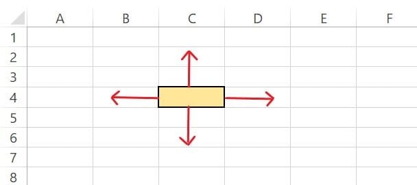
First of all, you should understand that with the help of the Excel OFFSET function, you can look up, down, left, and right.

Suppose my starting point is A1, and I want to go 4 cells down. I have to write a formula like this: =OFFSET(A1,4,0)

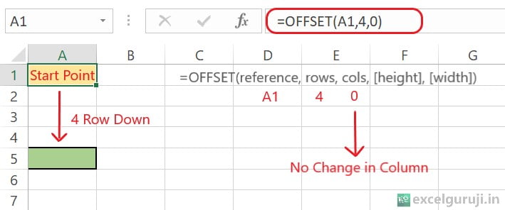
Now, let’s see how this formula works:

• The first part (reference) decides where it starts.
• The second part (rows), which is 4, moved down by 4 row.
• The third part (cols), which is 0, no change in column

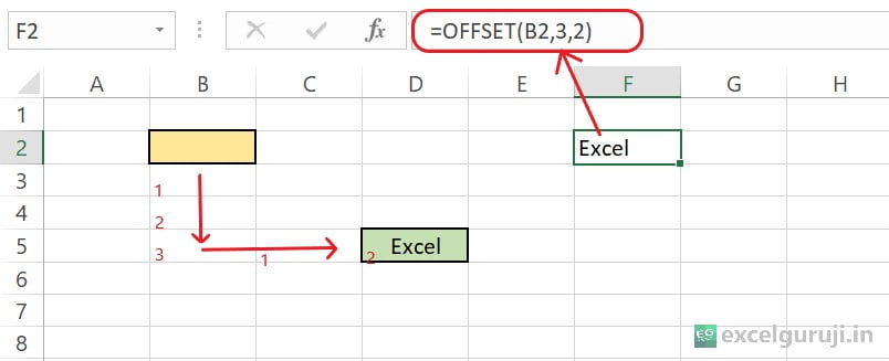
Now, suppose my starting point is the yellow cell (B2), and if I want to refer to the green cell (D5), then I have to write the formula like this.

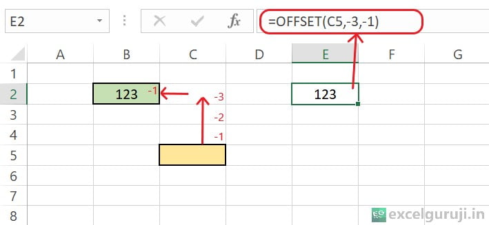
Now, let’s observe the impact by using negative values in the rows and columns arguments.

In the all above example, you saw how we used the necessary arguments (rows & cols) of the Excel OFFSET function. Now, let’s check out how to use the optional [height] and [width] arguments.

Imagine you want to use cell A1 (highlighted in yellow) as the reference and refer to the entire highlighted range in green (B3:D4) within a formula.

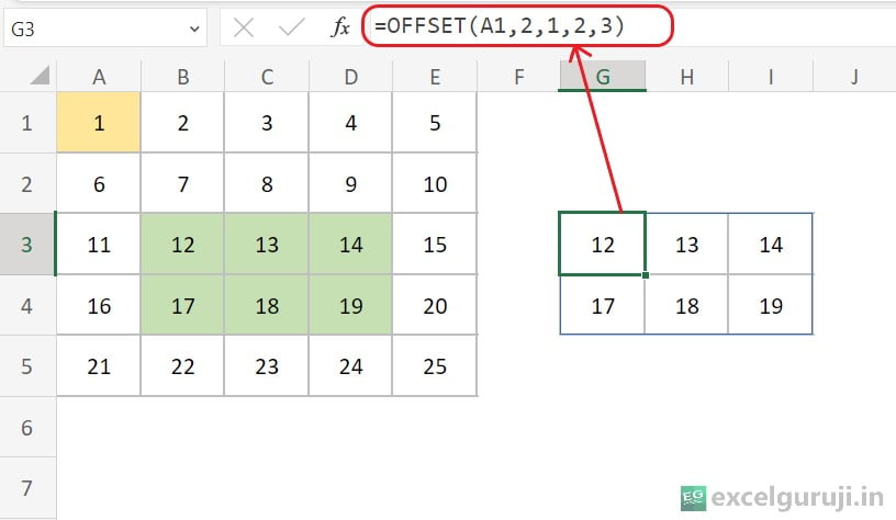
Now, let’s see how this formula works:

• The first part (reference) decides where it starts, which, in this case, is cell A1.
• The second part (rows), which is 2, moved down by 2 row.
• The third part (cols), which is 1, moved right by 1 column.
• The fourth part [height], which is 2, cover 2 rows.
• The fifth part [width], which is 3, cover 3 columns.

Note : It is important to note that if you are using a pre-dynamic array version (Excel 2019 and earlier), and you use the height and row arguments, you will encounter a #VALUE! error.

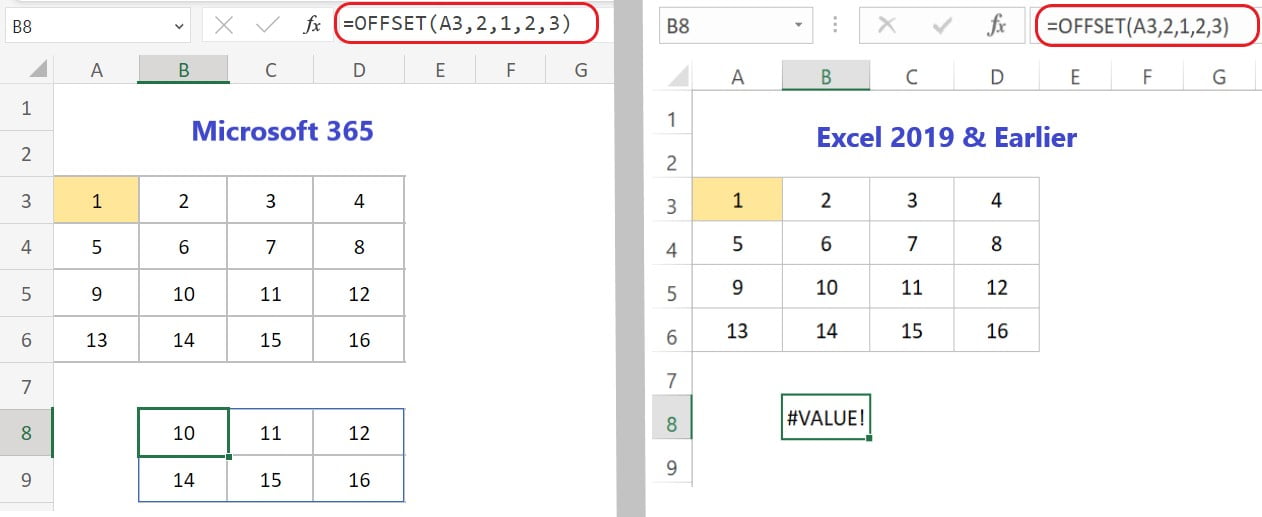
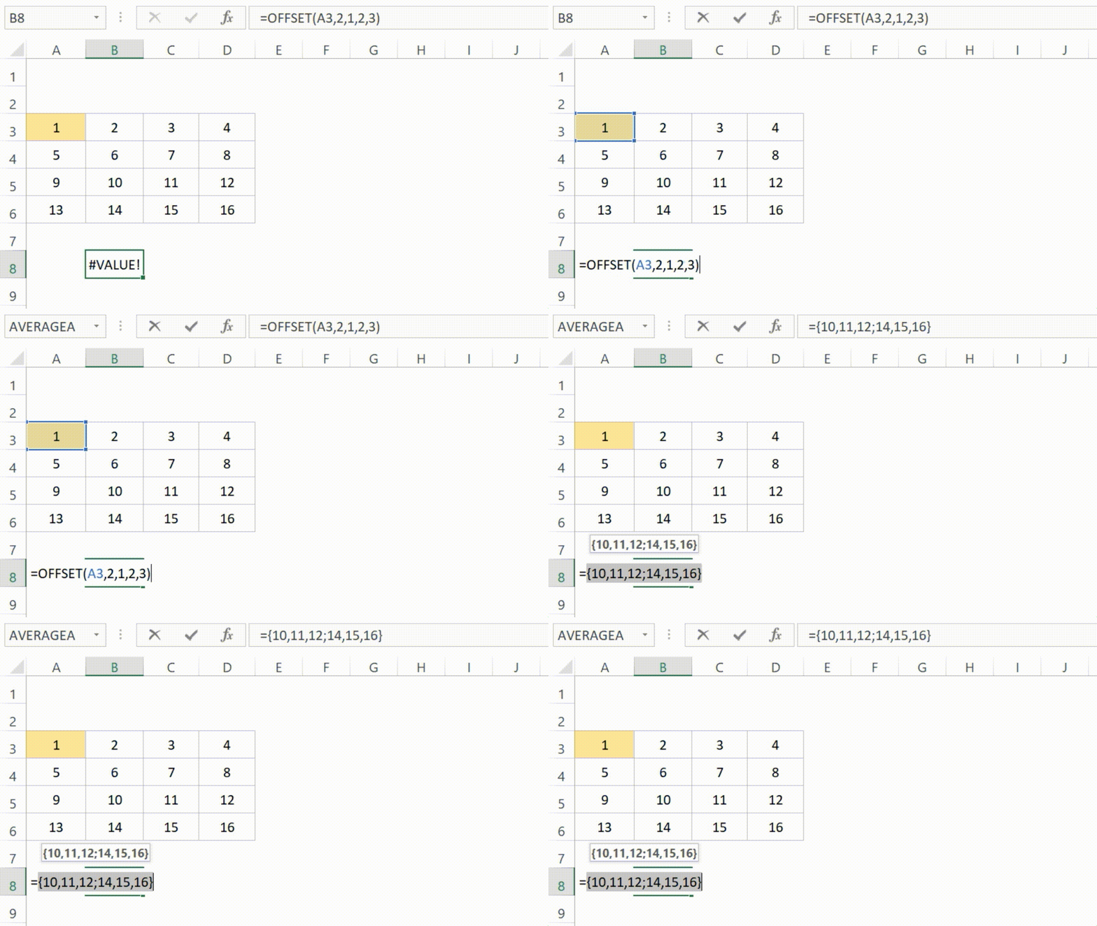
But don’t worry, you can still use the OFFSET function along with other functions even if there is an error. Just go to the cell’s edit mode, press F9, and you will see it gives you all the values it refers to in the formula.

Now, let’s say you want to add up all these values. You can easily do this by using the SUM function.

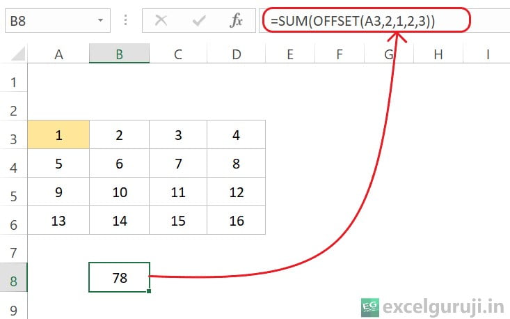
Hopefully, now you have a good idea of how to use the Excel OFFSET function. Let’s check out some real-life examples to make it even clearer.

Examples of the Excel OFFSET Function

Here are few examples of using the Excel OFFSET function in Excel:

Example 1: Find the Last Filled Cell

Imagine you have a list of numbers in column A, and you want to dynamically find the last filled cell in that column. Let’s explore how you can achieve this using the OFFSET function.

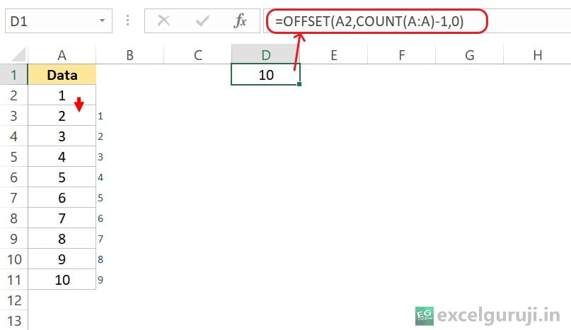
Here is an explanation of the formula: =OFFSET(A2,COUNT(A:A)-1,0)

• A2: This is the starting reference point for the OFFSET function. It begins counting from cell A2.
• COUNT(A:A)-1: This part determines the number of non-empty cells in column A. COUNT(A:A) counts all the cells in column A that have numbers in them. Subtracting 1 (-1) adjusts for the starting point A2. If you have numbers in cells A2 to A11, COUNT(A:A)-1 would be 10 – 1 = 9.
• 0: This is the number of columns to move to the right from the starting point (A2). Since it is 0, the OFFSET function stays in the same column.

Example 2: Drop Down that Adjusts Dynamically

You can apply the principles demonstrated in Example 1 to expand upon the idea and generate a dynamically adjusting drop-down list.

Imagine you are tasked with managing inventory of different fruits. And you want to create a dynamic drop-down list, and it automatically adjusts as you add or remove fruits name from the list in column A.

Here is an example of how it works:

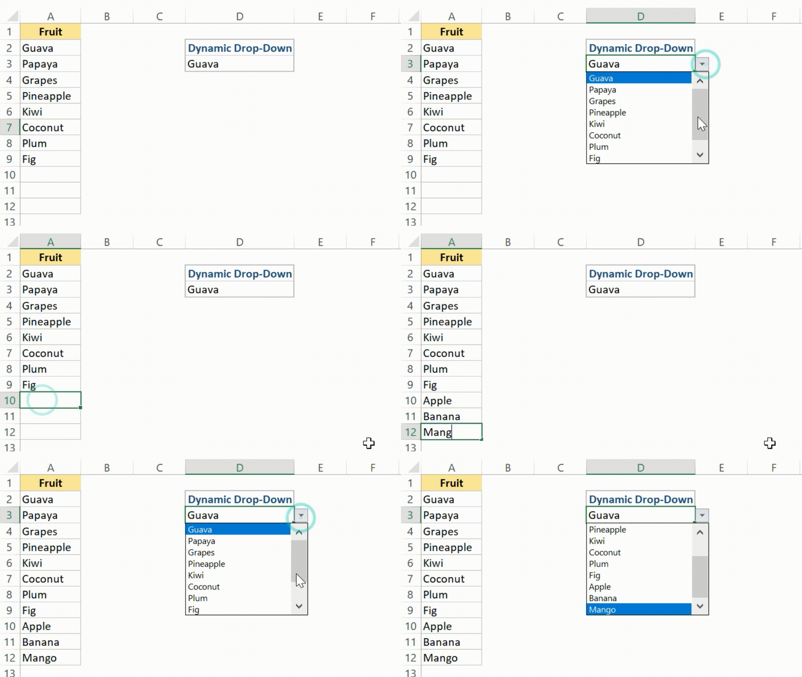
This happens because the formula used to make the drop-down is dynamic. It can figure out if you add or remove something and then adjust itself.

Here is how to make it work:

• Select the cell where you want the drop-down.
• Go to Data –> Data Tools –> Data Validation.

• In the Data Validation box, choose List from the options.

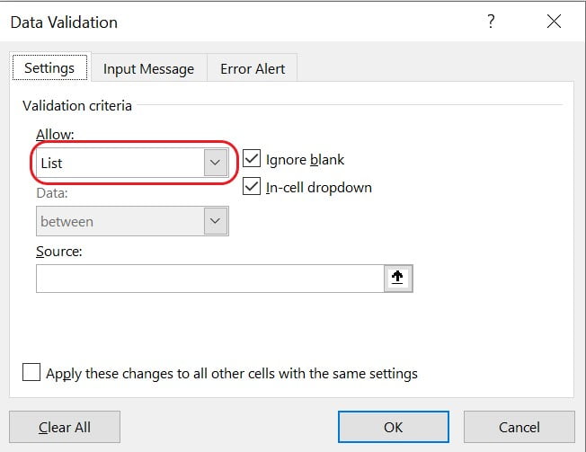
• In the source, type this formula: =OFFSET($A$2,0,0,COUNTA($A:$A),1), and Click OK

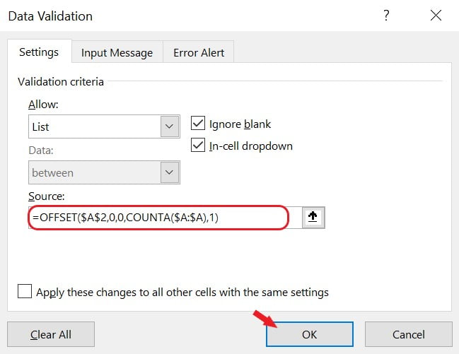
Let’s understand how this formula works:

• $A$2: This is the starting reference cell. The OFFSET function will use this cell as the starting point for the dynamic range.
• 0,0: These are the row and column offsets. In this case, both are set to 0, meaning there is no offset from the starting cell. The dynamic range starts from the cell specified in $A$2.
• COUNTA($A:$A): This part calculates the height of the range. COUNTA($A:$A) counts the number of non-empty cells in column A. It dynamically adjusts as you add or remove items from column A.
• 1: This represents the width of the range. In this case, it is set to 1, indicating that the dynamic range is one column wide.

Extra Notes

● Excel OFFSET function is a volatile functions (functions that recalculate with every change in the worksheet). This lead to performance issues and slow down your workbook.

● If the specified number of rows or columns is negative, the OFFSET function will reference cells above or to the left of the starting point.

● If the [height] and [width] arguments are omitted, the function returns a reference to a single cell.

● If the rows and columns offset the reference beyond the edge of the worksheet, OFFSET will show #REF! error.

● OFFSET doesn’t physically move cells or alter the selection, it simply gives a reference. You can pair OFFSET with any function that needs a reference.

Practice Workbook

Conclusion

In conclusion, the Excel OFFSET function is a versatile and powerful tool for dynamic referencing and data extraction. Whether you are building dynamic ranges, creating flexible models, or navigating through datasets, the OFFSET function can significantly enhance your Excel capabilities.

Remember, as with any Excel function, understanding its use and practicing in different scenarios will help you master the OFFSET function. Start incorporating OFFSET into your Excel toolkit today and open up new possibilities for dynamic data analysis.

Frequently Asked Questions (FAQs)

Q1: Can the Excel OFFSET function be used to reference a range from another sheet?

A1: Yes, the Excel OFFSET function can reference ranges from other sheets within the same workbook.

Q2: What happens if the specified rows or columns go beyond the boundaries of the worksheet?

A2: If the offset goes beyond the boundaries, Excel will return a #REF! error.

Q3: Can the OFFSET function be combined with other functions for advanced data analysis?

A3: Absolutely, the OFFSET function can be combined with various other functions, such as SUM, COUNT, AVERAGE, IF, etc. for advanced data analysis and modeling.

Q4: Are there any alternatives to the Excel OFFSET function for dynamic range creation?

A4: Yes, other functions like INDEX and INDIRECT can also be used for dynamic range creation, depending on the specific requirements of your workbook.

Other Related Excel Functions

Mastering Excel INDEX Function: A Guide to Dynamic Data Retrieval and Manipulation

Unleashing the Power of Excel INDIRECT Function: A Comprehensive Guide to Dynamic Cell Referencing

Mastering Excel VLOOKUP Function: A Comprehensive Guide to Enhance Your Data Analysis Skills

Unlocking Data Mastery with Excel HLOOKUP Function: A Comprehensive Guide for Efficient Horizontal Data Lookup

Mastering Excel FILTER Function: A Comprehensive Guide for Data Filtering

Join me on Instagram, YouTube and WhatApp Channel for your daily dose of valuable tips and tricks! Catch insightful videos that will enhance your knowledge and skills. Don’t miss out – follow me now!

1. OFFSET Function ↩︎