Mastering Excel LOOKUP Function: A Comprehensive Guide to Searching and Retrieving Data in Excel (With Practice File)

Excel LOOKUP Function

When to Use the Excel LOOKUP Function in Excel

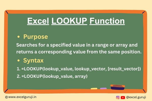
The LOOKUP function in Excel is a versatile tool used to search for a value in a range and return a corresponding value from the same position in another range. It is particularly handy when dealing with large datasets or when you need to quickly find specific information based on certain criteria.

What Excel LOOKUP Function Returns

The Excel LOOKUP function returns a value either from a one-row or one-column range or from an array. The function searches for the lookup_value in the first row or column of the specified range and returns the corresponding value from the same position in the last row or column of that range.

Syntax of Excel LOOKUP Function

The Excel LOOKUP function has two variations in syntax, and each serves a specific purpose:

Syntax 1:

=LOOKUP(lookup_value, lookup_vector, [result_vector])

This syntax is used when you want to find a value in a one-row or one-column range (lookup_vector) and return the corresponding value from another one-row or one-column range (result_vector). If result_vector is omitted, the function returns the corresponding value from lookup_vector.

Syntax 2:

=LOOKUP(lookup_value, array)

This syntax is employed when you want to find a value in an array and return the corresponding value from the same position in that array.

Input Arguments

Here are the input arguments for both variations of the Excel LOOKUP function:

● lookup_value: The value you want to search for in the lookup_vector or array.

● lookup_vector: For Syntax 1, this is the range that contains the values you want to compare with the lookup_value. It can be a one-row or one-column range or an array.

● result_vector: (Optional) For Syntax 1, this is the range that contains the values to be returned. If omitted, the function returns the corresponding value from the lookup_vector.

● array: For Syntax 2, this is the array in which you want to find the lookup_value.

Extra Notes

● The lookup_vector must be in ascending order. If it is not, the LOOKUP function may return #N/A/ error.

● If the lookup_value is smaller than the smallest value in the lookup_vector, the LOOKUP function returns the #N/A error.

● If the lookup_value is larger than the largest value in the lookup_vector, the LOOKUP function matches the largest value that is less than or equal to lookup_value.

● LOOKUP is not case-sensitive

Examples of the Excel LOOKUP Function

Here are few examples of using the LOOKUP function in Excel:

Example 1: Basic Usage

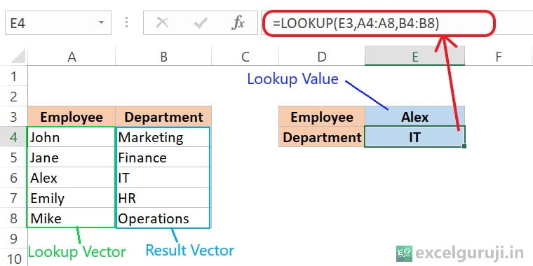
Imagine you are managing a small team, and you have a list of employees along with their respective departments. You receive a request to find the department for a specific employee. To accomplish this task, you decide to use the LOOKUP function in Excel.

Here is an explanation of the formula: =LOOKUP(E3,A4:A8,B4:B8)

• E3 contains the lookup value, which is “Alex” in this case.
• A4:A8 is the range where Excel will search for the lookup value. In this example, it is the range of employee names (John, Jane, Alex, Emily, Mike).
• B4:B8 is the range from which Excel will return the corresponding value. In this case, it is the range of departments (Marketing, Finance, IT, HR, Operations).

So, the formula is essentially saying, “Look for the value in cell E3 (‘Alex’) in the range A4:A8 (employee names), and return the corresponding value from the range B4:B8 (departments).

Example 2: Using an Array for Lookup

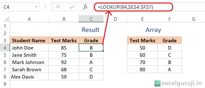
Imagine you are a teacher managing a class of students, and you have recently conducted a test. Each student’s test marks need to be graded. You have a list of students along with their respective test marks, and you want to use a lookup table to determine the corresponding grades. So, let us see in the following example how to use the LOOKUP function.

Here is an explanation of the formula: =LOOKUP(B4,$E$4:$F$7)

• B4 contains the test marks for a specific student, let’s say, Alex Davis, which is 59 in this case.
• $E$4:$F$7 represents the array table where Excel will look for the corresponding grade based on the test marks. The $ symbols before the column and row references make the range absolute, meaning it won’t change when you copy the formula to other cells.

So, the formula is saying, “Look for the value in cell B4 (test marks for Alex Davis) in the range of test marks in the array table (E4:E7), and return the corresponding grade from the second column of the array table (F4:F7).

Practice with Real Examples: Download the Attached Excel File

To facilitate your hands-on practice, I have attached an Excel file. You can download the file and work through the few examples I shared earlier, applying the LOOKUP function in Excel.

If you have any questions or need assistance, feel free to reach out. Enjoy practicing and mastering the Excel LOOKUP function!

Conclusion

In conclusion, the Excel LOOKUP function, with its two syntax variations, is an essential tool for quickly searching and retrieving information from a dataset. Whether you are working with product lists, employee data, or any other dataset, the LOOKUP function can streamline your tasks and make your Excel experience more efficient.

As with any Excel function, practice is key to mastering the LOOKUP function. Experiment with different scenarios and datasets to enhance your proficiency. Start using the LOOKUP function today and take your Excel skills to the next level!

Frequently Asked Questions (FAQs)

Q1: Can the LOOKUP function be used to search for values in multiple columns?

A1: Yes, the LOOKUP function can search for values in both one-row and one-column ranges, making it versatile for various data structures.

Q2: Is the Excel LOOKUP function case-sensitive?

A2: No, the Excel LOOKUP function is not case-sensitive.

Q3: What happens if the lookup_value is not found in the lookup_vector or array?

A3: In such cases, the LOOKUP function returns the #N/A error. You can use the IFERROR function to handle this situation and display a custom message.

Q4: Can the result_vector be in a different worksheet?

A4: Yes, the result_vector can be in a different worksheet. Simply reference the range using the appropriate worksheet notation.

Q5: Are there alternatives to the LOOKUP function for searching values in Excel?

A5: Yes, alternatives include functions like VLOOKUP, HLOOKUP, and INDEX-MATCH, each with its own advantages and use cases.

Other Related Excel Functions

Mastering Excel VLOOKUP Function: A Comprehensive Guide to Enhance Your Data Analysis Skills

Unlocking Data Mastery with Excel HLOOKUP Function: A Comprehensive Guide for Efficient Horizontal Data Lookup

Mastering Excel FILTER Function: A Comprehensive Guide for Data Filtering

Master Data Selection with Excel TAKE Function

Excel DROP Function: A Comprehensive Guide to Unlocking Excel’s Potential:

Join me on Instagram, YouTube and WhatApp Channel for your daily dose of valuable tips and tricks! Catch insightful videos that will enhance your knowledge and skills. Don’t miss out – follow me now!