Contents
Excel INDEX Function
When to Use the Excel INDEX Function in Excel
The INDEX function1 in Excel is a versatile tool designed for retrieving data from specific locations within a range, array, or reference. It offers dynamic solutions for data manipulation, making it an invaluable asset in scenarios where you need to work with tables, lists, or multiple ranges.
What Excel INDEX Function Returns
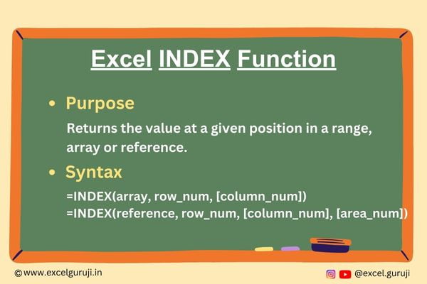
The Excel INDEX function returns the value of a cell in a specified range, array, or reference based on the row and column numbers provided as arguments.
Syntax of Excel INDEX Function
The Excel INDEX function has two syntax variations, depending on the type of data source:
Syntax 1: Syntax for Array or Range
=INDEX(array, row_num, [column_num])
This syntax is designed for situations where you are working with a single range or array of data.
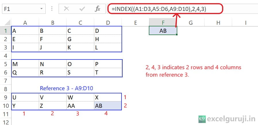
Syntax 2: Syntax for Reference with Multiple Areas:
=INDEX(reference, row_num, [column_num], [area_num])
This syntax is intended for cases where your data is organized into multiple non-contiguous ranges or areas. It enables you to reference a broader scope that consists of multiple areas, allowing you to retrieve data from specific rows and columns within those areas.
Input Arguments
Here are the input arguments for both variations of the Excel INDEX function:
● array: The range of cells, table, or array from which you want to retrieve the data.
● reference: The reference to a range that may consist of multiple areas. Such as (A1:C10, D7:F15).
● row_num: The row number within the reference from which to retrieve the data. It must be a positive integer.
● column_num: [Optional] The column number within the reference from which to retrieve the data. It must be a positive integer
Note: If you are using the Microsoft 365 version, setting the row_num & column_num argument to zero or leaving it blank (Omitted) will provide all rows and columns in the default array. However, in pre-dynamic array Excel (2019 and lower), you will receive a #VALUE! error in response.

● area_num: [Optional] The number of the area in reference from which to retrieve the data. If omitted, the function defaults to the first area.
Extra Notes
● If both row_num and column_num are provided, the function returns the value at the intersection of the specified row and column.
● If only row_num is provided, the function returns the entire row specified by that number (Only in the 365 version, the error will occur in the previous versions).
● If only column_num is provided, the function returns the entire column specified by that number (Only in the 365 version, the error will occur in the previous versions).
● #VALUE! error takes place when any of the provided row_num, column_num, or area_num arguments are non-numeric.
● It is essential that row_num and column_num and area_num arguments point to a cell within the array, otherwise, INDEX returns a #REF! error.
● If the array consists of only one row or column, the corresponding row_num or column_num argument becomes optional.
● In the scenario where the array has more than one row and more than one column, and only row_num or column_num is utilized, INDEX returns an array comprising the entire row or column in the array (Only in the 365 version, the error will occur in the previous versions).
Examples of the Excel INDEX Function
Here are few examples of using the Excel INDEX function in Excel:
Example 1: Basic Usage
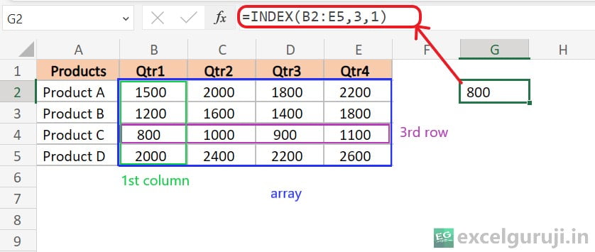
The Excel INDEX function retrieves a specific value from a range of cells based on its position. If the range is a single column or row, only a row or column number is required. However, for a two-dimensional range, both row and column numbers are necessary. You would use the formula like the following.
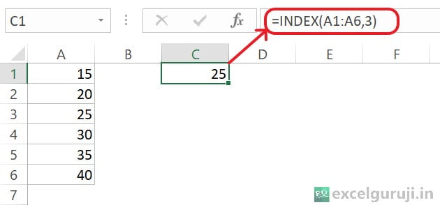
Now, The following formulas demonstrate how the Excel INDEX function can be employed to retrieve a value from a two-dimensional range:
Example 2: INDEX Function With MATCH Function
INDEX function and MATCH function are often used together in Excel due to their flexibility in dynamic data lookup, independence from column order, support for two-dimensional lookups, improved flexibility in changing lookup criteria, effectiveness with unsorted data, error handling capabilities, and the ability to function as array formulas, making them versatile tools in various data scenarios.
Suppose you have data on students and their grades, and you want to extract the grade with the help of the INDEX and MATCH functions. You can use the following formula:
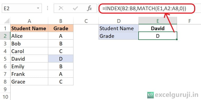
Here is an explanation of the formula: =INDEX(B2:B8,MATCH(E1,A2:A8,0))
- INDEX(B2:B8): This part of the formula refers to the range of grades (A, B, C, etc.), which is in column B from row 2 to row 8.
- MATCH(E1, A2:A8, 0): This part of the formula looks for the position of the value in cell E1 (which is “David” in this case) within the range A2:A8. The 0 in the MATCH function indicates an exact match.
- The MATCH function returns the relative position of the value in cell E1 within the range A2:A8. In this case, it returns 4 because “David” is in the fourth position in the list.
- Finally, INDEX uses this position (4) to retrieve the corresponding value from the range B2:B8, which is the grade associated with “David”. In your case, the grade is “D”.
So, the overall formula is finding the grade associated with the student name “David” and placing it in cell E2. If you change the value in cell E1 to another student name, the formula will dynamically retrieve the corresponding grade for that student.
In the above example, we used the MATCH function in place of the row_num argument. In the following example, we use the MATCH function in place of both the row_num and column_num arguments.
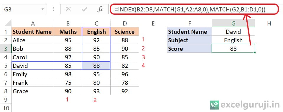
Here is an explanation of the formula: =INDEX(B2:D8,MATCH(G1,A2:A8,0),MATCH(G2,B1:D1,0))
- MATCH(G1, A2:A8, 0): Matches “David” in the range A2:A8, and returns the row position. In this case, it returns 4 because “David” is in the fourth row.
- MATCH(G2, B1:D1, 0): Matches “English” in the range B1:D1, and returns the column position. Here, it returns 2 because “English” is in the second column.
- INDEX(B2:D8, …, …): Uses the row and column positions obtained from the MATCH functions to index into the data range B2:D8. So, the final formula looks like this =INDEX(B2:D8,4,2)
Therefore, the formula returns the score of David in English, which is the value at the intersection of the fourth row and second column in the range B2:D8. In this case, it is 88.
Practice Workbook
Download Free Excel File For PracticeConclusion
In conclusion, the Excel INDEX function, with its two syntax variations, is a powerful tool for dynamic data retrieval and manipulation. Whether you are working with single arrays or referencing multiple areas across sheets, the Excel INDEX function provides a flexible solution for extracting specific data points based on specified criteria.
As you integrate the Excel INDEX function into your projects, you will find its versatility and functionality enhance your ability to handle diverse datasets and streamline your Excel workflows.
Frequently Asked Questions (FAQs)
Q1: Can the INDEX function retrieve data from multiple sheets?
A1: Yes, the INDEX function can be used to retrieve data from multiple sheets by referencing the appropriate sheet in the array argument.
Q2: Can the INDEX function handle non-numeric data?
A2: Absolutely, the INDEX function can handle both numeric and non-numeric data, making it suitable for various types of datasets.
Q3: What happens if the specified row or column number is outside the range of the array?
A3: If the specified row or column number is outside the range, the function may return an error.
Q4: Can the INDEX function be combined with other functions for more complex data manipulation?
A4: Yes, the INDEX function can be combined with other Excel functions to create more complex formulas for advanced data manipulation.
Q5: Is the INDEX function case-sensitive when working with text data?
A5: No, the INDEX function operates in a case-insensitive manner when working with text data.
Other Related Excel Functions
Mastering Excel VLOOKUP Function: A Comprehensive Guide to Enhance Your Data Analysis Skills
Mastering Excel FILTER Function: A Comprehensive Guide for Data Filtering
Join me on Instagram, YouTube and WhatApp Channel for your daily dose of valuable tips and tricks! Catch insightful videos that will enhance your knowledge and skills. Don’t miss out – follow me now!
1 thought on “Mastering Excel INDEX Function: A Guide to Dynamic Data Retrieval and Manipulation”