Taking this Excel Online Test 16 is more than just demonstrating what you know now, it is a chance for you to learn and grow. Each question is an opportunity to understand more.
Time's up
After you finish the Excel Online Test 16, we would really like it if you could tell us what you think. Share your thoughts, feedback, or even your score in the comments below. Your thoughts matter a lot to us. They help us make our content better for you. So, do your best, and when you’re done, take a moment to share your thoughts.
Being part of the excelguruji.in community is important to us, and we thank you for taking an active role!
Take the leap into Excel excellence! Click below to access our diverse quizzes, each crafted to push your skills to new heights. Your journey to becoming an Excel maestro starts here.
The TRANSPOSE function1 in Excel is a powerful tool used to change the orientation of a range of cells. It comes in handy when you need to switch rows to columns or vice versa. This function is particularly useful when working with data sets that require a different layout for analysis, reporting, or presentation purposes.
What Excel TRANSPOSE Function Returns
The Excel TRANSPOSE function returns a transposed range of cells, flipping the rows and columns of the specified data. It allows you to reorganize your data efficiently without manual copy-pasting or complex formulas.
Syntax of Excel TRANSPOSE Function
The syntax of the Excel TRANSPOSE function is as follows:
=TRANSPOSE(array)
Input Arguments
The Excel TRANSPOSE function has only one argument
● array: The range of cells or an array that you want to transpose. It can be a reference to a cell range, a range name, or an array constant.
Examples of the Excel TRANSPOSE Function
Here are few examples of using the Excel TRANSPOSE function in Excel:
Example 1:Basic Usage
Suppose you have data in the range A3:D6, and you want to switch the rows to columns or vice versa. In cell F3, input the following formula:
But, if you are using pre-dynamic array versions of Excel (Excel 2019 and earlier) and apply the formula described in the above example, you will encounter a #VALUE! error because they do not support array constants.
Now What?, you will find the solution in Example No. 2
Example 2:How to Use TRANSPOSE Function in Excel 2019 and Earlier Versions
First, count how many columns and rows are in the data you want to transpose
So, the data we want to TRANSPOSE has 4 columns and 5 rows.
Now, select some empty cells and make sure there are as many rows as the original table has columns and as many columns as the original table has rows.
Here, we select the same number of cells but they will be rotated from horizontal orientation to vertical, or vice versa.
After choosing some empty cells, type in the Transpose formula: =TRANSPOSE(A1:D5)
But wait, don’t press Enter just yet! Your Excel Transpose formula should look something similar like this:
To finish your formula correctly, press Ctrl + Shift + Enter.
After you press Ctrl + Shift + Enter, Excel will add {curly braces} around your Transpose formula. You will see them in the formula bar. Don’t try to type these braces yourself, it won’t work.
Look at the picture below. It shows that our original table has been successfully Transposed, turning 4 columns into 4 rows and 5 rows into 5 columns.
Example 3:TRANSPOSEWith Paste Special
The TRANSPOSE feature, also available in Paste Special, provides a non-formula approach to transpose data. Here is how to use this feature.
First, select the table you want to transpose and copy it. Then,
Right-click on the cell where you want to transpose the data and choose ‘Paste Special‘ or you can also use keyboard shortcut Ctrl + Alt + V
Now, the Paste Special dialog box will open.
Select ‘TRANSPOSE’ check box and click ‘OK.
So, now you can see that the copied part has been transposed successfully
Choosing Between TRANSPOSE Function and TRANSPOSE (Paste Special)
Now, you have two options available: one is the TRANSPOSE function, and the other is the TRANSPOSE Paste Special. You can choose the option that suits your requirements.
Dynamic Link vs. Static Data:
Use the TRANSPOSE function when you want a dynamic link between the original and transposed data.
Choose TRANSPOSE (Paste Special) when you need a one-time transformation and want the transposed data to be static.
Formula vs. Copy-Paste:
Use the TRANSPOSE function for a formula-based, dynamic transformation.
Choose TRANSPOSE (Paste Special) for a quick, non-formula, static rearrangement.
In conclusion, the Excel TRANSPOSE function is a valuable tool for quickly reorganizing your data, providing a more convenient way to analyze and present information. Whether you are dealing with small or large datasets, the TRANSPOSE function can save you time and effort by eliminating the need for manual rearrangement.
Experiment with the TRANSPOSE function in different scenarios to become proficient in its usage. As with any Excel function, practice is key to mastering its capabilities. Start incorporating the TRANSPOSE function into your projects today and enhance your data manipulation skills in Excel!
Frequently Asked Questions (FAQs)
Q1: Can the TRANSPOSE function be used with non-contiguous ranges?
A1: No, the TRANSPOSE function works best with contiguous ranges.
Q2: Does the TRANSPOSE function alter the original data?
A2: No, the TRANSPOSE function creates a transposed copy of the original data without modifying the original range.
Q3: Can the TRANSPOSE function be used with arrays created by formulas?
A3: Yes, the TRANSPOSE function can work with arrays generated by formulas, provided the resulting array is within the allowed limits.
Q4: What happens if the input range has different numbers of rows and columns?
A4: The TRANSPOSE function will not work correctly with ranges that do not have an equal number of rows and columns.
Q5: Are there any limitations to the size of the range that TRANSPOSE can handle?
A5: The size of the input range is limited by Excel’s overall size constraints, but for practical purposes, the TRANSPOSE function is suitable for a wide range of datasets.
Join me on Instagram, YouTube and WhatApp Channel for your daily dose of valuable tips and tricks! Catch insightful videos that will enhance your knowledge and skills. Don’t miss out – follow me now!
The TOROW function1 in Excel is a powerful tool designed for transposing data from a range or array into a single row. Whether you want to scan data by row or by column, the TOROW function provides flexibility and control over the transposition process.
What Excel TOROW Function Returns
The Excel TOROW function returns the specified array or range as a single row. It allows you to control the transposition process by choosing whether to ignore blank cells, errors, or both.
Syntax of Excel TOROW Function
The syntax of the Excel TOROW function is as follows:
=TOROW(array, [ignore], [scan_by_column])
Input Arguments
Here are the input arguments for the Excel TOROW function:
● array: The array or reference to be transposed into a single row.
● [ignore]: An optional argument that allows you to specify whether to ignore blank cells, errors, or both. The options are:
0: Keep all values (default)
1: Ignore blanks
2: Ignore errors
3: Ignore blanks and errors
● [scan_by_column]: An optional argument that determines whether the array is scanned by row (default) or by column.
If omitted or FALSE or 0, the array is scanned by row.
If TRUE or 1, the array is scanned by column.
Examples of the Excel TOROW Function
Here are few examples of using the Excel TOROW function in Excel:
Example 1:Basic Usage
Returns a single row from the array in the range A2:C5, scanned by row (default).
In the example above, we used only the array argument of the TOROW function. In this case, the TOROW function replaced the blank cell with zero, resulting in the data being displayed in a single row.
Example 2:Ignoring Blank Values
Now, let’s see how we can skip empty cells in a chosen array using the second [ignore] option in the TOROW function.
So, here we used 1 in the second argument. If you compare the previous result with the result of this formula =TOROW(A2:C5,1), you will notice that the empty cells have been eliminated from the array.
Example 3:Ignoring Error
Now, let’s explore how to exclude error values from the selected array.
So, when we put 2 in the [ignore] argument, it excludes the cell that has an error value.
Example 4:Ignoring Blanks & Error
Now, let’s see how we can skip both blank cells and cells with error values together using the second [ignore] option in the TOROW function.
So, by entering 3 in the [ignore] argument, we can skip both blank cells and cells with error values together.
Example 5:Scanning by Column
Excel’s TOROW function will, by default, scan the array horizontally (by row). However, if you want to scan vertically (by column), set the [scan_by_column] argument to TRUE.
See how, in both situations, the arrays are the same size, but the values are in a different order.
Extra Notes
● Excel TOROW function is exclusively accessible in Microsoft 365’s Excel and Excel for the web. It is not supported in pre-dynamic array versions of Excel (Excel 2019 and earlier) because they do not support array constants. To learn more about how to use Excel for Web for free. Watch 👇 this video
● The TOROWfunction provides flexibility by allowing you to choose whether to ignore blanks, errors, or both.
● Be cautious with large arrays, as Excel may return a #NUM error if the array is too large.
Time to Apply Your Knowledge.
Take a hands-on approach to mastering the Excel TOROW function. Utilize the provided Excel file to experiment and witness its functionality with sample data.
Should you have any questions or stumble upon intriguing insights, don’t hesitate to share your thoughts in the comments. Embrace the learning journey with practical experience!
Conclusion
In conclusion, the Excel TOROW function is a valuable tool for efficiently transposing data into a single row. Whether you need to adjust the layout of your data for reporting or analysis, the TOROW function provides the flexibility and control you need.
Start incorporating the TOROW function into your Excel projects today to streamline your data manipulation tasks and enhance your spreadsheet proficiency.
Frequently Asked Questions (FAQs)
Q1: Can the TOROW function transpose data from a column into multiple rows?
A1: No, the TOROW function is designed specifically for transposing data from a column into a single row, not for transforming data into multiple rows.
Q2: How does the TOROW function handle blank cells and errors?
A2: The TOROW function provides options to ignore blank cells, errors, or both. By adjusting the [ignore] argument, you can customize how the function treats these elements during transposition.
Q3: What happens if the array is too large?
A3: If the array is excessively large, Excel may return a #NUM error. It is advisable to manage the size of your array to prevent this issue.
Q4: Can I use the TOROW function with non-contiguous data?
A4: Yes, you have the option to merge the ranges into a single array using the VSTACK function, and afterward, apply TOROW to convert the merged array into a row.
Join me on Instagram, YouTube and WhatApp Channel for your daily dose of valuable tips and tricks! Catch insightful videos that will enhance your knowledge and skills. Don’t miss out – follow me now!
The TOCOL function1 in Excel is a powerful tool designed for transposing data from a range or array into a single column. Whether you want to scan data by row or by column, the TOCOL function provides flexibility and control over the transposition process.
What Excel TOCOL Function Returns
The Excel TOCOL function returns the specified array or range as a single column. It allows you to control the transposition process by choosing whether to ignore blank cells, errors, or both.
Syntax of Excel TOCOL Function
The syntax of the Excel TOCOL function is as follows:
=TOCOL(array, [ignore], [scan_by_column])
Input Arguments
Here are the input arguments for the Excel TOCOL function:
● array: The array or reference to be transposed into a single column.
● [ignore]: An optional argument that allows you to specify whether to ignore blank cells, errors, or both. The options are:
0: Keep all values (default)
1: Ignore blanks
2: Ignore errors
3: Ignore blanks and errors
● [scan_by_column]: An optional argument that determines whether the array is scanned by row (default) or by column.
If omitted or FALSE or 0, the array is scanned by row.
If TRUE or 1, the array is scanned by column.
Examples of the Excel TOCOL Function
Here are few examples of using the Excel TOCOL function in Excel:
Example 1:Basic Usage
Returns a single column from the array in the range A2:C5, scanned by row (default).
In the example above, we used only the array argument of the TOCOL function. In this case, the TOCOL function replaced the blank cell with zero, resulting in the data being displayed in a single column.
Example 2:Ignoring Blank Values
Now, let’s see how we can skip empty cells in a chosen array using the second [ignore] option in the TOCOL function.
So, here we used 1 in the second argument. If you compare the previous result with the result of this formula =TOCOL(A2:C5,1), you will notice that the empty cells have been eliminated from the array.
Example 3:Ignoring Error
Now, let’s explore how to exclude error values from the selected array.
So, when we put 2 in the [ignore] argument, it excludes the cell that has an error value.
Example 4:Ignoring Blanks & Error
Now, let’s see how we can skip both blank cells and cells with error values together using the second [ignore] option in the TOCOL function.
So, by entering 3 in the [ignore] argument, we can skip both blank cells and cells with error values together.
Example 5:Scanning by Column
Excel’s TOCOL function will, by default, scan the array horizontally (by row). However, if you want to scan vertically (by column), set the [scan_by_column] argument to TRUE.
See how, in both situations, the arrays are the same size, but the values are in a different order.
Extra Notes
● Excel TOCOL function is exclusively accessible in Microsoft 365’s Excel and Excel for the web. It is not supported in pre-dynamic array versions of Excel (Excel 2019 and earlier) because they do not support array constants. To learn more about how to use Excel for Web for free. Watch 👇 this video
● The TOCOL function provides flexibility by allowing you to choose whether to ignore blanks, errors, or both.
● Be cautious with large arrays, as Excel may return a #NUM error if the array is too large.
Time to Apply Your Knowledge.
Take a hands-on approach to mastering the Excel TOCOL function. Utilize the provided Excel file to experiment and witness its functionality with sample data.
Should you have any questions or stumble upon intriguing insights, don’t hesitate to share your thoughts in the comments. Embrace the learning journey with practical experience!
Conclusion
In conclusion, the Excel TOCOL function is a valuable tool for efficiently transposing data into a single column. Whether you need to adjust the layout of your data for reporting or analysis, the TOCOL function provides the flexibility and control you need.
Start incorporating the TOCOL function into your Excel projects today to streamline your data manipulation tasks and enhance your spreadsheet proficiency.
Frequently Asked Questions (FAQs)
Q1: Can the TOCOL function be used to transpose data from a row into a column?
A1: No, the TOCOL function is designed specifically for transposing data from a column into a single column, not for transforming data from a row.
Q2: How does the TOCOL function handle blank cells and errors?
A2: The TOCOL function provides options to ignore blank cells, errors, or both. By adjusting the [ignore] argument, you can customize how the function treats these elements during transposition.
Q3: What happens if the array is too large?
A3: If the array is excessively large, Excel may return a #NUM error. It is advisable to manage the size of your array to prevent this issue.
Q4: Can I use the TOCOL function with non-contiguous data?
A4: Yes, you have the option to merge the ranges into a single array using the VSTACK function, and afterward, apply TOCOL to convert the merged array into a column.
Join me on Instagram, YouTube and WhatApp Channel for your daily dose of valuable tips and tricks! Catch insightful videos that will enhance your knowledge and skills. Don’t miss out – follow me now!
The SORTBY function1 in Excel is a powerful tool used for sorting data based on the values in a specified range or array. It comes in handy when you need to arrange your data dynamically, allowing you to prioritize information based on specific criteria.
What Excel SORTBY Function Returns
The Excel SORTBY function returns a sorted array or range based on the values in another corresponding array or range. It helps you organize your data in ascending or descending order, making it easier to analyze and interpret.
Syntax of Excel SORTBY Function
The syntax of the Excel SORTBY function is as follows:
Here are the input arguments for the Excel SORTBY function:
● array: The range or array of values that you want to sort.
● by_array1: The range or array of values based on which you want to sort the main array.
● sort_order1: Optional. Specifies the sort order for the corresponding by_array1 (1 for ascending, -1 for descending).
● by_array2, sort_order2, …: Optional. Additional ranges or arrays and their corresponding sort orders for more complex sorting criteria.
Examples of the Excel SORTBY Function
Here are few examples of using the Excel SORT function in Excel:
Example 1:Basic Sorting
Suppose you have a list of countries in column A, and you want to sort them by their sales values in ascending order. In cell D2, you can use the following formula:
Let’s break down the formula: =SORTBY(A2:A13,B2:B13)
A2:A13: This is the array or range of values that you want to sort.
B2:B13: This is the by_array or range of values based on which you want to sort the main array (A2:A13). It could represent sales values, quantities, or any other criteria you want to use for sorting. The values in B2:B13 will determine the order of the corresponding values in A2:A13.
Example 2:Multi-level Sorting
Imagine you have a table with names in column A, ages in column B, and you want to sort the table first by age in ascending order and then by name in descending order. In cell D2, you can use the following formula:
This formula sorts the table based on age in ascending order and then on name in descending order.
Extra Notes
● Excel SORTBY function is exclusively accessible in Microsoft 365’s Excel and Excel for the web. It is not supported in pre-dynamic array versions of Excel (Excel 2019 and earlier) because they do not support array constants. To learn more about how to use Excel for Web for free. Watch 👇 this video
● The SORTBY function is dynamic, meaning that if the values in the by_array change, the sorted result will automatically update.
● If there are ties in the sort criteria, SORTBY maintains the original order of those tied items.
● Make sure all the lists you are sorting have the same size, or SORTBY might give you an error (#VALUE!).
Time to Apply Your Knowledge.
Take a hands-on approach to mastering the Excel SORTBY function. Utilize the provided Excel file to experiment and witness its functionality with sample data.
Should you have any questions or stumble upon intriguing insights, don’t hesitate to share your thoughts in the comments. Embrace the learning journey with practical experience!
Conclusion
In conclusion, the Excel SORTBY function is a versatile tool for dynamically sorting data based on specified criteria. Whether you are working with simple lists or complex datasets, SORTBY can streamline your data analysis tasks and enhance your efficiency in Excel.
Remember, mastering Excel functions takes practice, so don’t hesitate to experiment with different sorting criteria and explore the full potential of the SORTBY function in your projects. Start utilizing the SORTBY function today and take your Excel skills to new heights!
Frequently Asked Questions (FAQs)
Q1: Can the SORTBY function sort data in both ascending and descending order?
A1: Yes, by providing the appropriate sort_order argument, you can specify whether the sorting should be in ascending (1) or descending (-1) order.
Q2: Can the SORTBY function handle multiple sorting criteria?
A2: Yes, the SORTBY function supports multi-level sorting by allowing you to specify multiple arrays and their corresponding sort orders.
Q3: Does the SORTBY function automatically update when the data changes?
A3: Yes, the SORTBY function is dynamic, and if the values in the by_array change, the sorted result will automatically update.
Q4: What happens if there are ties in the sorting criteria?
A4: If there are ties, the SORTBY function maintains the original order of those tied items.
Q5: Is the Excel SORTBY function suitable for large datasets?
A5: Yes, the Excel SORTBY function is particularly useful for handling large datasets and complex sorting requirements in Excel.
Join me on Instagram, YouTube and WhatApp Channel for your daily dose of valuable tips and tricks! Catch insightful videos that will enhance your knowledge and skills. Don’t miss out – follow me now!
The SORT function1 in Excel is a powerful tool that comes in handy when you need to arrange the data in a specific order. Whether you are dealing with numerical values, dates, or text, the SORT function allows you to organize your data in ascending or descending order, making it easier to analyze and draw insights.
What Excel SORT Function Returns
The Excel SORT function returns a sorted array or range based on the specified criteria. It can be applied to both single columns and multiple columns, providing flexibility in sorting data according to your requirements.
Syntax of Excel SORTFunction
The syntax of the Excel SORT function is as follows:
Here are the input arguments for the Excel SORT function:
● array: The range or array that you want to sort.
● sort_index: (Optional) The column or row index by which to sort the array. If omitted, the function uses the first column.
● sort_order: (Optional) The order in which to sort the array. Use 1 for ascending order (default) or -1 for descending order.
● by_col: (Optional) A logical value that specifies whether to sort by columns (TRUE) or rows (FALSE). If omitted, the default is FALSE.
Examples of the Excel SORT Function
Here are few examples of using the Excel SORT function in Excel:
Example 1:Basic Sorting
In the following example, you will see that we have used only the first argument of the SORT function, which is an array(A2:D13)
By default, the Excel SORT function will sort the first column of the selected array (A2:D13) in ascending order.
Example 2:Sorting by a Specific Column
As we saw in the example above, just by providing the area argument, it takes the first column and sorts it. But if you have more columns, you can sort the data by specifying the column number, The SORT function below sorts by the fourth column.
Note: Make changes only to the formula in cell F2. Excel will handle the rest.
Example 3:Sorting in Descending Order
Now, we use the sort_order argument (the third part of the formula) in SORT function to put the data in descending order. The formula below sorts the array based on the fourth column, from biggest to smallest.
We used -1 for the sort_order argument to arrange the data in descending order.
Example 4:Sorting on multiple columns
To sort by multiple columns, just provide an array. For example, you can sort first by Country and then by Sales.
Example 5:Advanced Sorting on Multiple Columns
The advanced SORT function below showcases a sophisticated sorting approach. It begins by sorting data based on Country in ascending order, providing a primary level of organization. Subsequently, it fine-tunes the sorting criteria by incorporating Sales in descending order as a secondary parameter.
This two-step sorting process demonstrates the versatility and advanced capabilities of the SORT function in Excel.
Suppose you have a dataset containing quarterly sales information for various countries in different regions, and your goal is to extract and sort data specifically for Qtr 2 sales. You can use the following formula:
Let’s break down the formula: =SORT(FILTER(A2:D13, C2:C13=”Qtr 2″), 4)
FILTER(A2:D13, C2:C13=”Qtr 2″): This part of the formula filters the data in the range A2:D13 based on the condition specified in C2:C13. It selects only the rows where the value in column C is equal to “Qtr 2”. So, it filters out the rows that don’t match the condition, effectively creating a subset of the original data.
SORT(…, 4): This part of the formula takes the result of the FILTER function and sorts it based on the values in the fourth column D (Sales) in ascending order by default. The number ‘4’ indicates the column number by which to sort.
Extra Notes
● Excel SORT function is exclusively accessible in Microsoft 365’s Excel and Excel for the web. It is not supported in pre-dynamic array versions of Excel (Excel 2019 and earlier) because they do not support array constants. To learn more about how to use Excel for Web for free. Watch 👇 this video
● If the sort_index argument is beyond the valid range, the SORT function returns a #VALUE! error.
● Additionally, if any cells within the spill range are not entirely blank or are merged, a #SPILL! error occurs. To resolve this issue, simply clear any obstructions in the affected cells.
Time to Apply Your Knowledge.
Take a hands-on approach to mastering the Excel FILTER function. Utilize the provided Excel file to experiment and witness its functionality with sample data.
Should you have any questions or stumble upon intriguing insights, don’t hesitate to share your thoughts in the comments. Embrace the learning journey with practical experience!
Conclusion
In conclusion, the Excel SORT function is a valuable tool for organizing and arranging data in a systematic manner. Whether you are dealing with simple lists or complex tables, the SORT function provides a versatile solution for customizing the order of your data.
Remember, exploring and experimenting with the SORT function in different scenarios will enhance your proficiency in Excel. Start incorporating the SORT function into your projects today, and streamline the way you analyze and present your data.
Frequently Asked Questions (FAQs)
Q1: Can the SORT function be used for sorting alphanumeric data?
A1: Yes, the SORT function can handle both numeric and text values, providing a comprehensive sorting solution.
Q2: Is it possible to sort data based on multiple columns?
A2: Absolutely, you can specify multiple columns for sorting.
Q3: What happens if the sort_index exceeds the number of columns in the array?
A3: If the specified sort_index is greater than the number of columns in the array, the function returns a #VALUE! error.
Q4: Can the SORT function be used to sort data in a specific order, such as a custom list?
A4: The SORT function primarily sorts data in ascending or descending order. If you need a custom sort order, additional techniques or helper columns may be required.
Q5: Does the SORT function modify the original data, or does it create a new sorted array?
A5: The SORT function returns a new array with the sorted data and does not modify the original data.
Join me on Instagram, YouTube and WhatApp Channel for your daily dose of valuable tips and tricks! Catch insightful videos that will enhance your knowledge and skills. Don’t miss out – follow me now!
Participating in this Excel Online Test 15 extends beyond showcasing your current knowledge, it serves as a platform for personal growth. Each question offers an opportunity to expand your comprehension.
Time's up
After completing the Excel Online Test 15, we would greatly appreciate it if you could share your insights, feedback, or even your achieved score in the comments section below. Your input is incredibly valuable to us, helping enhance and tailor our content to better meet your needs. So, give it your best effort, and once you have finished, please take a moment to provide us with your thoughts.
Your presence within the excelguruji.in community is highly valued, and we sincerely thank you for actively participating!
Ready for the next Excel challenge? Click below to explore our quiz collection, designed to elevate your skills. Whether you are a beginner or an advanced user, there is always more to discover.
The OFFSET function1 in Excel proves to be a powerful tool when you need to dynamically reference a range of cells based on a starting point and a specified number of rows and columns. It is particularly handy for creating dynamic ranges, performing complex calculations, and building flexible data analysis models.
What Excel OFFSET Function Returns
The Excel OFFSET function returns a reference to a range that is offset from a starting reference point. The offset is determined by the specified number of rows and columns.
Syntax of Excel OFFSET Function
The syntax of the Excel OFFSET function is as follows:
=OFFSET(reference, rows, cols, [height], [width])
Input Arguments
Here are the input arguments for the Excel OFFSET function:
● reference: The starting point or reference cell from which the offset will be applied. This can be a cell reference or a named range.
● rows: The number of rows to offset from the reference. If you use a positive number, it moves down rows. If you use a negative number, it goes up rows. If you keep zero, then there is no change.
● cols: The number of columns to offset from the reference. If you use a positive number, it moves right columns. If you use a negative number, it moves left columns. If you keep zero, then there is no change.
● [height]: (Optional) The height of the range to be returned. If omitted, the function returns a single cell. Positive or negative numbers can be used; however, if you keep it as zero, a #REF! error will occur.
● [width]: (Optional) The width of the range to be returned. If omitted, the function returns a single cell. Positive or negative numbers can be used; however, if you keep it as zero, a #REF! error will occur.
Learning the Basics of Excel OFFSET
The Excel OFFSET function may seem confusing at first, but once you delve into its details, you will discover its ease of use, allowing you to incorporate it systematically into your formulas.
Now, let’s explore how this function operates:
First of all, you should understand that with the help of the Excel OFFSET function, you can look up, down, left, and right.
Suppose my starting point is A1, and I want to go 4 cells down. I have to write a formula like this: =OFFSET(A1,4,0)
Now, let’s see how this formula works:
The first part (reference) decides where it starts.
The second part (rows), which is 4, moved down by 4 row.
The third part (cols), which is 0, no change in column
Now, suppose my starting point is the yellow cell (B2), and if I want to refer to the green cell (D5), then I have to write the formula like this.
Now, let’s observe the impact by using negative values in the rows and columns arguments.
In the all above example, you saw how we used the necessary arguments (rows & cols) of the Excel OFFSET function. Now, let’s check out how to use the optional [height] and [width] arguments.
Imagine you want to use cell A1 (highlighted in yellow) as the reference and refer to the entire highlighted range in green (B3:D4) within a formula.
Now, let’s see how this formula works:
The first part (reference) decides where it starts, which, in this case, is cell A1.
The second part (rows), which is 2, moved down by 2 row.
The third part (cols), which is 1, moved right by 1 column.
The fourth part [height], which is 2, cover 2 rows.
The fifth part [width], which is 3, cover 3 columns.
Note : It is important to note that if you are using a pre-dynamic array version (Excel 2019 and earlier), and you use the height and row arguments, you will encounter a #VALUE! error.
But don’t worry, you can still use the OFFSET function along with other functions even if there is an error. Just go to the cell’s edit mode, press F9, and you will see it gives you all the values it refers to in the formula.
Now, let’s say you want to add up all these values. You can easily do this by using the SUM function.
Hopefully, now you have a good idea of how to use the Excel OFFSET function. Let’s check out some real-life examples to make it even clearer.
Examples of the Excel OFFSET Function
Here are few examples of using the Excel OFFSET function in Excel:
Example 1:Find the Last Filled Cell
Imagine you have a list of numbers in column A, and you want to dynamically find the last filled cell in that column. Let’s explore how you can achieve this using the OFFSET function.
Here is an explanation of the formula: =OFFSET(A2,COUNT(A:A)-1,0)
A2: This is the starting reference point for the OFFSET function. It begins counting from cell A2.
COUNT(A:A)-1: This part determines the number of non-empty cells in column A. COUNT(A:A) counts all the cells in column A that have numbers in them. Subtracting 1 (-1) adjusts for the starting point A2. If you have numbers in cells A2 to A11, COUNT(A:A)-1 would be 10 – 1 = 9.
0: This is the number of columns to move to the right from the starting point (A2). Since it is 0, the OFFSET function stays in the same column.
Example 2:Drop Down that Adjusts Dynamically
You can apply the principles demonstrated in Example 1 to expand upon the idea and generate a dynamically adjusting drop-down list.
Imagine you are tasked with managing inventory of different fruits. And you want to create a dynamic drop-down list, and it automatically adjusts as you add or remove fruits name from the list in column A.
Here is an example of how it works:
This happens because the formula used to make the drop-down is dynamic. It can figure out if you add or remove something and then adjust itself.
Here is how to make it work:
Select the cell where you want the drop-down.
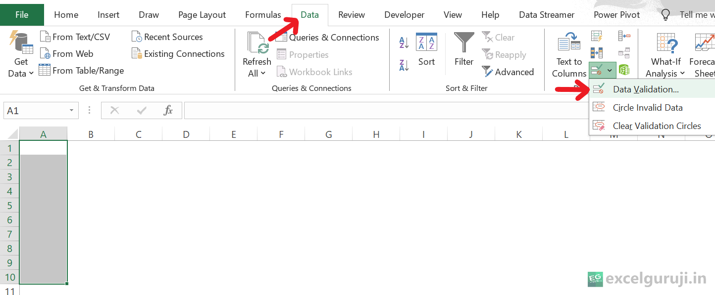
Go to Data –> Data Tools –> Data Validation.
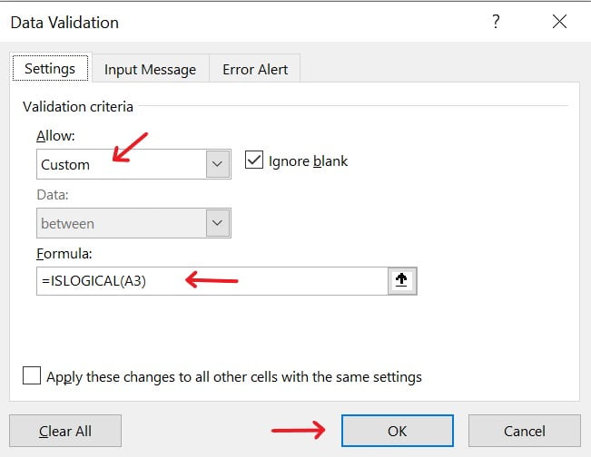
In the Data Validation box, choose List from the options.
In the source, type this formula: =OFFSET($A$2,0,0,COUNTA($A:$A),1), and Click OK
Let’s understand how this formula works:
$A$2: This is the starting reference cell. The OFFSET function will use this cell as the starting point for the dynamic range.
0,0: These are the row and column offsets. In this case, both are set to 0, meaning there is no offset from the starting cell. The dynamic range starts from the cell specified in $A$2.
COUNTA($A:$A): This part calculates the height of the range. COUNTA($A:$A) counts the number of non-empty cells in column A. It dynamically adjusts as you add or remove items from column A.
1: This represents the width of the range. In this case, it is set to 1, indicating that the dynamic range is one column wide.
Extra Notes
● Excel OFFSET function is a volatile functions (functions that recalculate with every change in the worksheet). This lead to performance issues and slow down your workbook.
● If the specified number of rows or columns is negative, the OFFSET function will reference cells above or to the left of the starting point.
● If the [height] and [width] arguments are omitted, the function returns a reference to a single cell.
● If the rows and columns offset the reference beyond the edge of the worksheet, OFFSET will show #REF! error.
● OFFSET doesn’t physically move cells or alter the selection, it simply gives a reference. You can pair OFFSET with any function that needs a reference.
In conclusion, the Excel OFFSET function is a versatile and powerful tool for dynamic referencing and data extraction. Whether you are building dynamic ranges, creating flexible models, or navigating through datasets, the OFFSET function can significantly enhance your Excel capabilities.
Remember, as with any Excel function, understanding its use and practicing in different scenarios will help you master the OFFSET function. Start incorporating OFFSET into your Excel toolkit today and open up new possibilities for dynamic data analysis.
Frequently Asked Questions (FAQs)
Q1: Can the Excel OFFSET function be used to reference a range from another sheet?
A1: Yes, the Excel OFFSET function can reference ranges from other sheets within the same workbook.
Q2: What happens if the specified rows or columns go beyond the boundaries of the worksheet?
A2: If the offset goes beyond the boundaries, Excel will return a #REF! error.
Q3: Can the OFFSET function be combined with other functions for advanced data analysis?
A3: Absolutely, the OFFSET function can be combined with various other functions, such as SUM, COUNT, AVERAGE, IF, etc. for advanced data analysis and modeling.
Q4: Are there any alternatives to the Excel OFFSET function for dynamic range creation?
A4: Yes, other functions like INDEX and INDIRECT can also be used for dynamic range creation, depending on the specific requirements of your workbook.
Join me on Instagram, YouTube and WhatApp Channel for your daily dose of valuable tips and tricks! Catch insightful videos that will enhance your knowledge and skills. Don’t miss out – follow me now!
The INDIRECT function1 in Excel proves invaluable when you need to dynamically reference cells or ranges. It allows you to create flexible and dynamic formulas by converting text representations of cell references or named ranges into actual references.
What Excel INDIRECT Function Returns
The Excel INDIRECT function returns the value of the referenced cell or range specified by a text string. This enables you to construct formulas that can change dynamically based on the contents of a cell.
Syntax of Excel INDIRECT Function
The syntax of the Excel INDIRECT function is as follows:
=INDIRECT(ref_text, [a1])
Input Arguments
Here are the input arguments for the Excel INDIRECT function:
● ref_text: This is the reference text that you want to convert into an actual cell reference or a named range. It can be a text string enclosed in quotation marks, a cell reference, or the result of another formula.
● [a1]: This is an optional argument that determines the reference type. If omitted or set to TRUE, the reference is interpreted in A1 style (column letter and row number). If set to FALSE, the reference is interpreted in R1C1 style (row and column number).
Extra Notes
● If the ref_text argument refers to a cell on another sheet, that sheet must be open, or the INDIRECT function will return a #REF! error.
● Excel INDIRECT function is a volatile functions (functions that recalculate with every change in the worksheet). This lead to performance issues and slow down your workbook.
● The ref_text argument can include the sheet name followed by an exclamation mark to specify a cell or range on a different sheet.
Examples of the Excel INDIRECT Function
Here are few examples of using the Excel INDIRECR function in Excel:
Example 1:Basic Usage
Suppose you have data in cell A1, and you want to retrieve the value from that cell using the INDIRECT function. You just need to provide it with the name of the cell, written as text, as shown in the example below.
Here is an explanation of the formula: =INDIRECT(“A1”)
The formula above accepts the cell reference A1 as an input argument (enclosed in double quotes as a text string) and yields the value found in that cell, which, in this case, is 100.
Now, you might be wondering if this could have been achieved by directly referencing the sales (e.g., A1 or =$A$1), as demonstrated below. Then, why should we use the INDIRECT function unnecessarily?
When you use =A1 or =$A$1, you get the same result. But, if you add a row above the first row, the cell references change automatically to fit the new row.
When adding rows or columns to a worksheet and needing to keep the cell reference locked and unchanged, you can utilize the Excel INDIRECT function.
Example 2:Use Cell Reference
Suppose you have data in cell A1, and you want to dynamically reference the cell specified in cell C1. In cell E1, you can use the following formula:
When you use the Excel INDIRECT function with C1 (which holds a cell address as text), it makes A1 a proper reference. This means it looks at A1 and gives you what is there.
Remember, no need for quotes because C1 has the cell address in text.
But if C1 has something that is not a proper cell address, INDIRECT will show an error (#REF!).
You can make a reference to a cell by using both the column letter and the row number. For example, if you have the number 1 in cell C1, and you use the formula =INDIRECT(“A” & C1), it will point to cell A1, as shown in the example below.
Example 3:Calculate the Average of a Range of Cells
You can use the Excel INDIRECT function in Excel to reference a range of cells, just as you would reference a single cell, as shown in the example below.
Here is an explanation of the formula: =AVERAGE(INDIRECT(“A1:A6”))
INDIRECT(“A1:A6”): The INDIRECT function is used to convert the text string “A1:A6” into a reference to the actual range A1 to A6. So, it essentially refers to the range of cells A1 to A6.
AVERAGE(INDIRECT(“A1:A6”)): The AVERAGE function then calculates the average of the numbers in the range A1 to A6.
Just like the AVERAGE function, you can use other functions such as SUM, COUNT, MAX, MIN, LARGE, SMALL, etc.
Example 4:INDIRECT Function With Name Range
When Excel INDIRECT function combined with named ranges, it can be a powerful tool for creating dynamic and flexible formulas. Named ranges allow you to assign a meaningful name to a specific cell or range of cells, making it easier to understand and manage your formulas.
Suppose you have the following data on test scores for students in different subjects:
The scores for the subjects are listed in columns B, C, and D. To make it easier to refer to these ranges, you can assign names to them. Specifically, you want to name the range in column B as “Math” the range in column C as “Science”, and the range in column D as “English”.
Now, to achieve this, you can follow the method below:
Select the Range:
Highlight the cells in column B where the Math scores are (e.g., B2 to B7).
Then, go to the “Formulas” tab on the ribbon.
Click on “Define Name” or “Name Manager” (depending on your Excel version).
Enter the name “Math” and click OK. Now, the range B2:B7 is named as “Maths”.
Repeat the same process for Other Subjects:
Now, you can use the Excel INDIRECT function to refer to the named range in a formula.
For example, if you want to average the values in the named range “Math” you could use the following formula:
Example 5:Dependent Drop-down List with the Excel INDIRECT Function
Creating a dependent dropdown list in Excel using the INDIRECT function involves setting up named ranges and using data validation.
For example, suppose you have a list of categories arranged in a row and their corresponding subcategories in a column, as shown below:
Now, to create a dependent dropdown list, assign a name range to each category, such as A2:A6 for Electronics, B2:B6 for Clothing, and C2:C6 for Furniture. We have already covered how to assign name ranges in the previous example.
Now, select the cell where you want to create a dropdown list for the main category (Electronics, Clothing, Furniture). This will be the first drop-down list.
Select cell E2
Click on Data Tab
Click on Data Validation
Select List as the Validation criteria and use the following formula in the Source field: =$A$1:$C$1
Your first drop-down list will look like below:
Now follow below method to create dependable drop-down list:
Select cell F2
Click on Data Tab
Click on Data Validation
Select List as the Validation criteria and use the following formula in the Source field: =$A$1:$C$1
Now, when you select ‘Electronics’ in the first drop-down (cell E2), the dependent drop-down in cell F2 will display the subcategories of Electronics (Phones, Laptops, Headphones, Smartwatches, Digital Cameras).
And when you select ‘Furniture’ in the first drop-down, the dependent drop-down in cell F2 will display the subcategories of Furniture (Tables, Sofas, Chairs, Beds, Dining Sets).
In conclusion, the Excel INDIRECT function is a powerful tool for creating dynamic and flexible formulas. It enables you to build formulas that adapt to changes in your spreadsheet, providing a level of versatility that static cell references cannot achieve.
As with any Excel function, it is essential to understand the nuances and potential pitfalls of the INDIRECT function. Experiment with different applications to enhance your proficiency and efficiency in utilizing this function in your Excel projects.
Frequently Asked Questions (FAQs)
Q1: Can the INDIRECT function reference cells on other sheets?
A1: Yes, by including the sheet name followed by an exclamation mark in the ref_text argument.
Q2: What happens if the referenced sheet is not open?
A2: If the referenced sheet is not open, the INDIRECT function will return a #REF! error.
Q3: What is the purpose of the [a1] argument?
A3: The [a1] argument determines the reference type. If TRUE or omitted, the reference is interpreted in A1 style; if FALSE, in R1C1 style.
Q4: Is there a performance impact when using the INDIRECT function with volatile functions?
A4: Yes, using the INDIRECT function with volatile functions can lead to performance issues.
Join me on Instagram, YouTube and WhatApp Channel for your daily dose of valuable tips and tricks! Catch insightful videos that will enhance your knowledge and skills. Don’t miss out – follow me now!
The MATCH function1 in Excel comes in handy when you need to:
● Locate the position of a specific value in a range. ● Check if a value exists in a list or array. ● Determine the relative position of an item in a sorted or unsorted list.
What Excel MATCHFunction Returns
The Excel MATCH function returns the relative position of a specified value in a range. The result can be one of three values:
● If the function finds an exact match, it returns the position of the item. ● If no match is found, it returns the #N/A error. ● If the match type is set to 1 and the data is not sorted, it returns the position of the nearest value less than or equal to the lookup value.
Syntax of Excel MATCHFunction
The syntax of the Excel MATCH function is as follows:
=MATCH(lookup_value, lookup_array, [match_type])
Input Arguments
Here are the input arguments for the Excel MATCH function:
● lookup_value: The value you want to find in the lookup_array.
● lookup_array: The range of cells containing possible matches.
● match_type: An optional argument that specifies the type of match. It can be 1 (less than), 0 (exact match), or -1 (greater than).
Match Type Behavior:
1 or Omitted: If no exact match is found, the function returns the position of the closest value less than the lookup value. The lookup array must be sorted in ascending order.
0: If no exact match is found, the function returns an error. The lookup array does not need to be sorted.
-1: If no exact match is found, the function returns the position of the closest value greater than the lookup value. The lookup array must be sorted in descending order.
Extra Notes
● MATCH is not case-sensitive.
● When no match is found, MATCH returns the #N/A error.
● MATCH is limited to working with text strings of up to 255 characters in length.
● If there are duplicate values, MATCH returns the position of the first occurrence.
● For match_type values of -1 or 1, it is essential for the lookup_array to be sorted, as mentioned earlier.
Examples of the Excel MATCH Function
Here are few examples of using the Excel MATCH function in Excel:
Example 1:Basic Usage
Suppose you have a list of fruits names in column A, and you want to find the position of the fruit “Pear” in the list. In cell D3, use the following formula:
Here is an explanation of the formula: =MATCH(D2,A3:A11,0)
D2: This is the lookup_value. In this case, it is “Pear”, and the formula is trying to find the position of “Pear” within the specified range.
A3:A11: This is the lookup_array. It represents the range of cells where Excel will search for the value “Pear”.
0: This is the match_type. The value 0 indicates that the function should find an exact match.
Example 2:Less Than Match
Suppose you have a set of numbers, and you want to find the position of the largest number less than the given lookup value. So, you need to select 1 for the match_type argument and write the MATCH function as shown below:
So, in the above example, we observe that the largest value below lookup_value (475), i.e., the number 400, is located at the fourth position. As mentioned earlier, we have arranged the lookup_array (A3:A12) in ascending order (smallest to largest) to obtain the correct result.
Example 3:Greater Than Match
Suppose you have a set of numbers, and you want to find the position of the smallest number greater than a given lookup value. So, you need to select -1 for the match_type argument and write the MATCH function as shown below:
So, in the above example, we observe that the smallest value above lookup_value (475), i.e., the number 500, is located at the sixth position. As mentioned earlier, we have arranged the lookup_array (A3:A12) in descending order (largest to smallest) to obtain the correct result.
Example 4:INDEX Function With MATCH Function
INDEX Function and MATCH Function are like a dynamic duo in Excel. They team up to search for data in a flexible way. They don’t mind how the columns are arranged, can hunt for data in both rows and columns, easily adapt to different criteria, handle unsorted data well, manage errors gracefully, and can be used as array formulas. This makes them versatile and powerful tools for handling various data situations in Excel.
I highly recommend reading my previous INDEX function post for a deeper understanding of this concept.
In conclusion, the Excel MATCH function is a valuable tool for locating specific values in a range. Whether you are working with lists of data, managing inventories, or analyzing information, the MATCH function can streamline your tasks and improve your Excel proficiency.
As with any Excel function, it’s essential to understand the syntax and experiment with different scenarios to master its usage. Start incorporating the MATCH function into your Excel projects today to enhance your data analysis and decision-making capabilities.
Frequently Asked Questions (FAQs)
Q1: Can the MATCH function be used to find the position of the last occurrence of a value?
A1: No, the MATCH function returns the position of the first occurrence of a value.
Q2: Is the MATCH function case-sensitive?
A2: No, the MATCH function is not case-sensitive.
Q3: What does the #N/A error mean in the context of the MATCH function?
A3: The #N/A error is returned when no match is found for the specified lookup value.
Q4: Can the Excel MATCH function handle arrays as lookup arrays?
A4: Yes, the Excel MATCH function can handle arrays as lookup arrays, making it versatile for various data structures.
Join me on Instagram, YouTube and WhatApp Channel for your daily dose of valuable tips and tricks! Catch insightful videos that will enhance your knowledge and skills. Don’t miss out – follow me now!