How to Create a Drop Down List in Excel

Drop down lists are like magic boxes in Excel – they offer pre-defined choices, making data entry a breeze and reducing errors. This guide, explains everything you need to know about drop down lists.

Video Tutorial – How to create a drop down list in Excel

What are Drop Down Lists in Excel?

Imagine a cell in your spreadsheet. Instead of typing things in every time, you want users to choose from a specific set of options. That is where drop down lists come in! They display a small arrow, and clicking it reveals a list of choices users can select.

Benefits:

1. Faster and easier data entry: No more typing the same things repeatedly!

2. Reduced errors: Users can only choose from pre-defined options, minimizing typos and inconsistencies.

3. Improved data consistency: Ensures everyone uses the same terms and values.

How to Create Drop Down List in Excel?

There are several ways to create drop down lists, depending on how you have your data organized:

1. Entering choices manually

2. Using range of cells

3. Using named ranges

4. Using formula (Dynamic drop down list)

By Entering Choices Manually

For example, if you wish to create a drop down list within a cell with three options, Yes and No, here is how you can input manually them directly into the data validation source field.

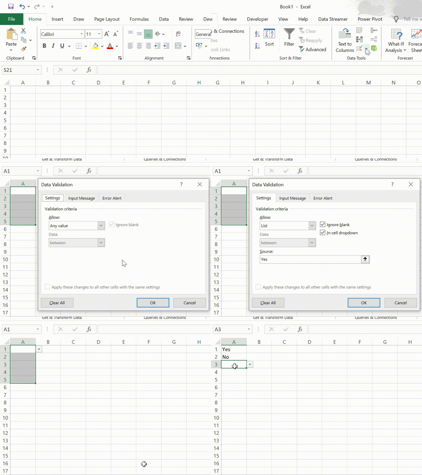
1. Choose the cell where you want the drop down list. It can be a single cell, a range of cells, a whole column, or non-continuous cells. (To select non-continuous cells, press the Ctrl key and then select each desired cell.)

2. Go to the “Data” tab on the top ribbon.

3. Click the “Data Validation” button in the “Data Tools” ribbon.

4. In the Data Validation window, choose the “Settings” tab.

5. From the Allow drop down menu, select “List”.

6. Type your list of choices separated by commas (with or without spaces), like “Yes, No“

7. Click “OK” to save and activate the drop down list.

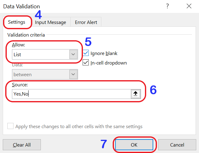
Note: Ensure that the “In-cell drop down” option is checked (which is the default setting); otherwise, the drop down arrow will not appear next to the cell.

By Using Range of Cells

If you have a predefined list of options in a separate range of cells, you can reference that range to create your drop down list.

Follow the same steps as above, but instead of manually entering the options, select the range containing the data you want to use.

1. Make a separate list of options somewhere on your sheet.

2. Choose the cell where you want the drop down list.

3. Go to the “Data” tab on the top ribbon.

4. Click the “Data Validation” button in the “Data Tools” ribbon.

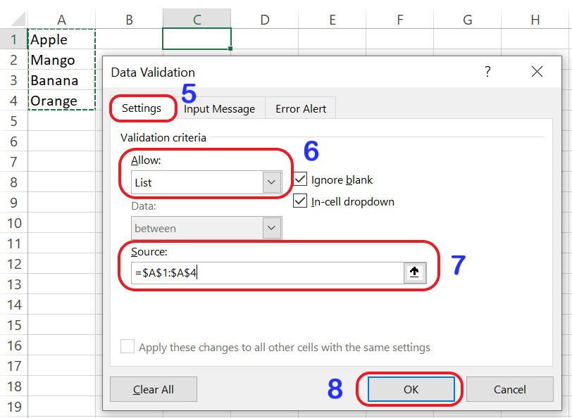
5. In the Data Validation window, choose the “Settings” tab.

6. From the Allow drop down menu, select “List”.

7. Enter the cell range of your list in the “Source” box.

8. Click “OK” to save and activate the drop down list.

By Using Name Range

Named ranges provide a convenient way to refer to a specific range of cells by a custom name.

Define a named range for your list of options, and then use that name when setting up data validation to create your drop down list.

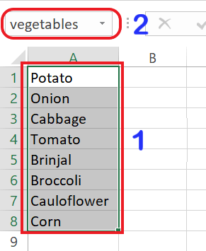
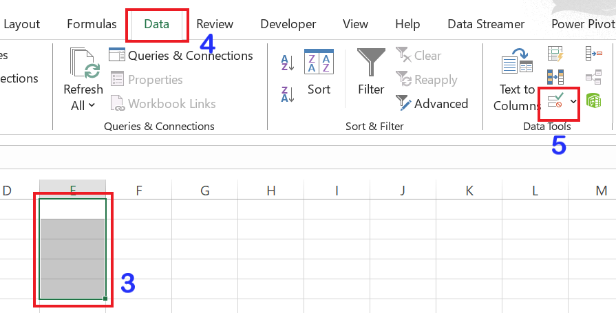
1. Select a cell or group of cells you wish to assign a name to.

2. Enter a name in the Name Box and press Enter key

For example, let’s name the range ‘vegetables’.

3. Choose the cell where you want the drop down list.

4. Go to the “Data” tab on the top ribbon.

5. Click the “Data Validation” button in the “Data Tools” ribbon.

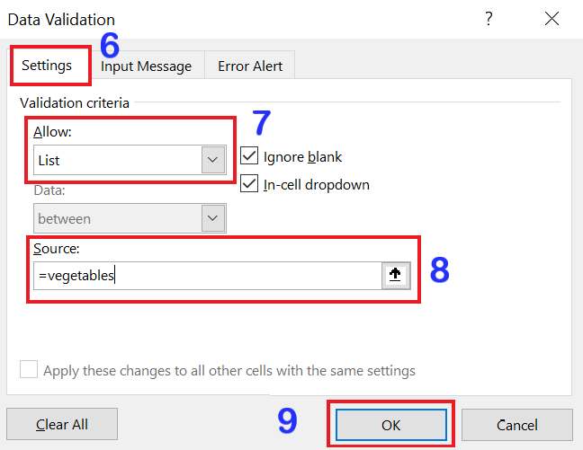
6. In the Data Validation window, choose the “Settings” tab.

7. From the Allow drop down menu, select “List”.

8. Enter the name range as =vegetables in the “Source” box.

9. Click “OK” to save and activate the drop down list.

Tips💡: When you insert multiple drop downs in different sheets, using named ranges makes them easier to identify and manage

Create Dynamic Drop Down List

Static drop down lists are useful, but sometimes you need them to adjust dynamically based on changes in the source data. This is where dynamic drop down lists come into play.

By leveraging Excel’s functions like OFFSET, you can create drop down lists that automatically update as your data changes.

Below is the method for creating a dynamic drop down:

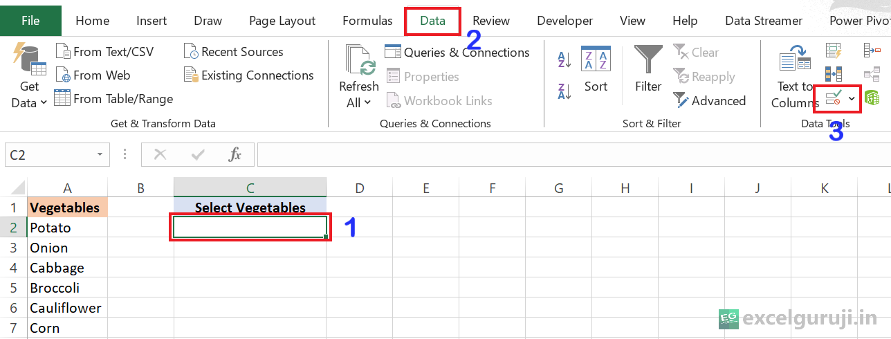
1. Choose the cell where you want the drop down list. It can be a single cell, a range of cells, a whole column, or non-continuous cells. (To select non-continuous cells, press the Ctrl key and then select each desired cell.)

2. Go to the “Data” tab on the top ribbon.

3. Click the “Data Validation” button in the “Data Tools” ribbon.

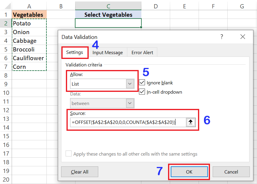
4. In the Data Validation window, choose the “Settings” tab.

5. From the Allow drop down menu, select “List”.

6. Use the following formula in the source field: =OFFSET($A$2:$A$20,0,0,COUNTA($A$2:$A$20))

7. Click “OK” to save and activate the drop down list.

Benefits of this formula:

The formula automatically adjusts the size of the drop down list based on the number of entries in your data.

If you add or remove items in A2:A20, the drop down list will update accordingly.

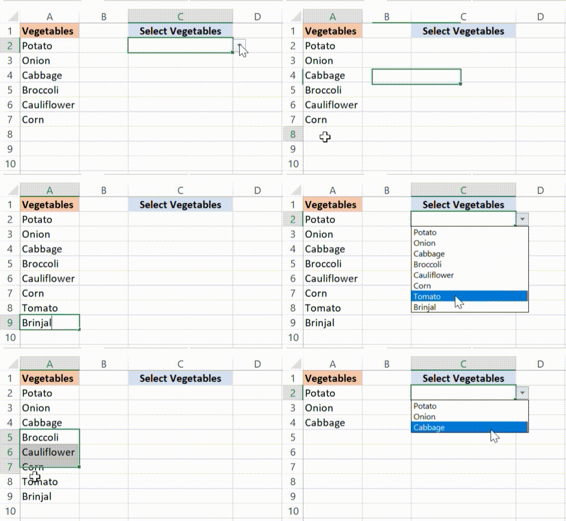
Here is a breakdown of how this formula works: =OFFSET($A$2:$A$20,0,0,COUNTA($A$2:$A$20))

The syntax of the Excel OFFSET function is: =OFFSET(reference, rows, cols, [height], [width])

The syntax of the Excel COUNTA function is: =COUNTA(value1, [value2], …)

OFFSET: This function returns a reference to a range that is offset from a starting cell or range of cells by a specified number of rows and columns. It is commonly used for dynamic range references.

$A$2:$A$20: This is the starting range. In this case, it is the range of cells from A2 to A20. This is the range from which the drop down list values will be derived. The dollar signs ($) make the reference absolute, meaning it won’t change if you copy the formula to another cell.

0, 0: These are the number of rows and columns by which the range specified in the first argument (A2:A20) will be offset. Here, both are set to 0, meaning there is no offset. This indicates that the drop down list will start from the first cell of the specified range.

COUNTA($A$2:$A$20): This function counts the number of non-empty cells in the range A2:A20. It is used here to dynamically determine the height of the range for the drop down list. This ensures that the drop down list only includes non-empty cells within the specified range.

Note: To make sure it works, there shouldn’t be any empty cell between the filled cells.

Create a Dependable Drop Down List

A dependable drop down list is where the options in a second drop down are adjusted based on the selection made in the first.

Below is the example of dependable drop down list

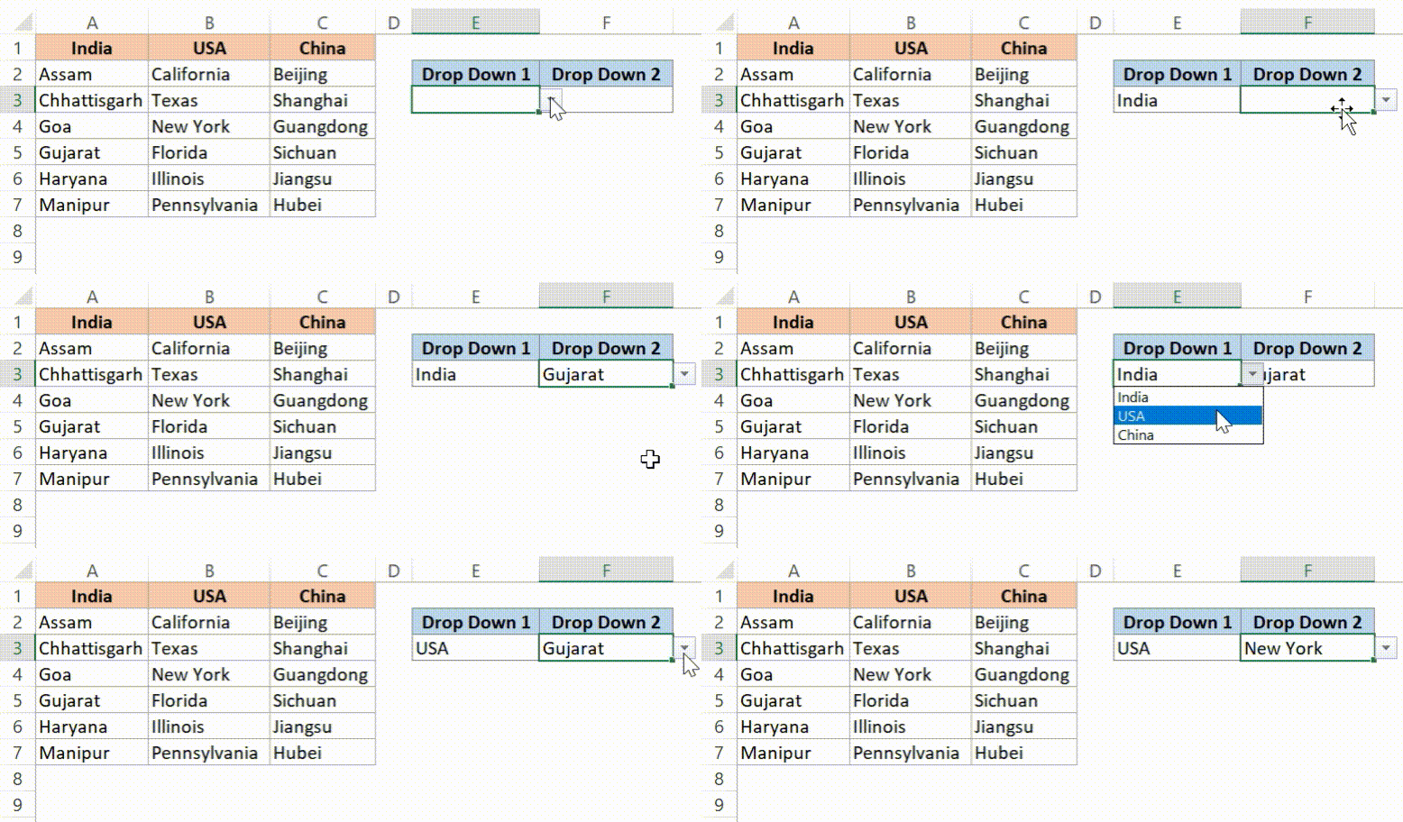
In the example above, the options in ‘Drop Down 2’ change based on what you pick in ‘Drop Down 1’.

Now, let’s see how to do this.

Here are the steps to make a drop down list in Excel that changes depending on what you pick:

◼ Select the cell where you want your first drop down list.

◼ Click the “Data” tab and then “Data Validation”

◼ In the Data Validation window, choose the “Settings” tab.

◼ From the Allow drop down menu, select “List”.

◼ Enter the range of your first drop down list.

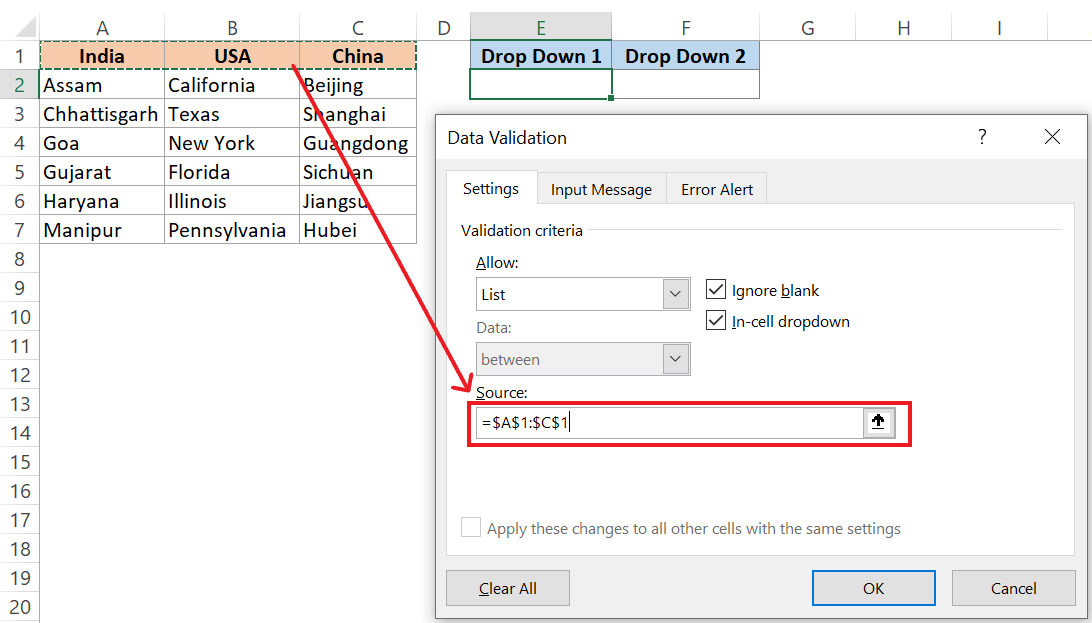
◼ Click “OK” to save and activate the drop down list.

◼ Now, your first drop down list is ready

◼ To create a second drop down list, first create individual named ranges for each country in the top row, follow these steps:

◼ Select the entire list of states, including the country names in the top row.

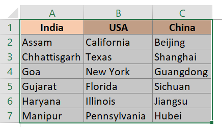
◼ Go to the “Formulas” tab and click “Create from Selection”. (Alternatively, you can use keyboard shortcut Ctrl + Shift + F3)

◼ In the “Create Names from Selection” dialogue box, only check the “Top row” option and leave all other options unselected.

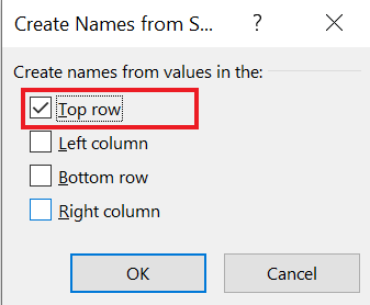
◼ Click “OK”.

This will create a separate named range for each country name in the top row. For example, the range named “India” will refer to all the states listed under the country “India” in the list.

◼ Select the cell where you want your second drop down list.

◼ Click the “Data” tab and then “Data Validation”.

◼ In the Data Validation window, choose the “Settings” tab.

◼ From the Allow drop down menu, select “List”.

◼ Enter a name range using the INDIRECT function, like =INDIRECT(E2), in the “Source” box. Cell E2 contains the first drop down list.

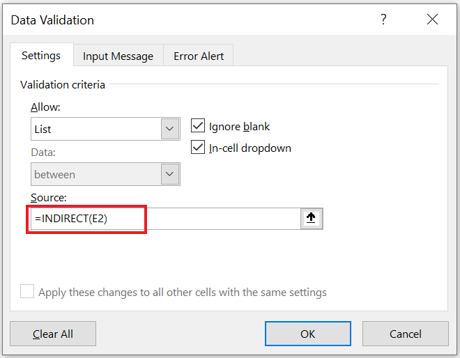
◼ Click “OK”.

When you choose something from the first drop down list (cell E2), the options in the second list (cell F2) will automatically change.

Why does this happen? Because the second list uses a special formula that looks at the first list. When you pick “India” in the first list, the second list knows to show you only the states within India, thanks to the magic of a function called INDIRECT.

Important Note

If your first list has names with spaces (like “United States of America”), you need a special trick. Excel doesn’t like spaces in its names, so it replaces them with underscores when you create named ranges. For example, “United States of America” becomes “United_States_of_America”.

To make the drop down list work with such names, we use a helper function called SUBSTITUTE. It simply replaces the spaces in your choice with underscores before checking the named range, making everything work smoothly.

You need to use this formula =INDIRECT(SUBSTITUTE(E2,” “,”_”))

Create a Drop Down From Another Worksheet

Excel allows you to reference data from other worksheets within the same workbook, making it easy to create drop down lists that pull options from different sheets.

There are three ways to create a drop down list that uses data from another sheet:

Named Range: Give your list in another sheet a name (like “Countries”). Then, when setting up the drop down list, use the name instead of the cell range. Make sure the name applies to the entire workbook, not just the sheet it is in.

Excel Table: Simply use the table name when setting up the drop down list. Excel tables work across different sheets without needing extra steps.

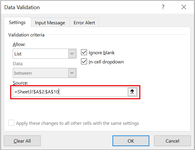
Regular Range: When using a regular cell range from another sheet, you need to include the sheet name in the reference. For example, if your list is in sheet “Sheet3” on cell range A1:A10, the reference would be “Sheet3!A1:A10”. Excel will automatically add the sheet name when you select the range.

Create a Drop Down From Another Workbook

Expanding on the previous method, Excel also allows you to reference data from external workbooks to create drop down lists.

This can be particularly useful when collaborating with colleagues or consolidating data from multiple sources. Follow these steps to create a drop down list from another workbook:

In the file with the list (source file):

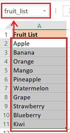
◼ Give your list a name range, like “fruit_list”.

In the file where you want the drop down menu:

◼ Click the “Formulas” tab and then “Define Name”.

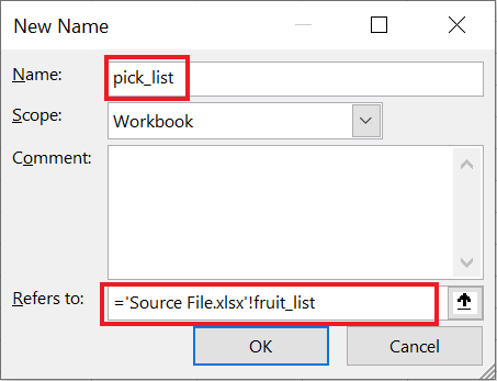
◼ Give another name range, like “pick_list”, to a special reference that points to your list in the source file. This reference will look something like =SourceFile.xlsx!fruit_list.

Tip: If the source file name has spaces or special characters, put quotes around it, like =’Source File.xlsx’!fruit_list. (Like in our example)

◼ Click “OK”.

◼ Choose the cell for your drop down menu and go to the “Data” tab.

◼ Click the “Data” tab and then “Data Validation”.

◼ In the Data Validation window, choose the “Settings” tab.

◼ From the Allow drop down menu, select “List”.

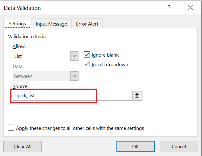
◼ In the “Source” box, type the name range you gave the reference in step 2 (e.g., “=pick_list”).

◼ Click “OK”.

Things to keep in mind:

◼ Both files need to be open for the drop down menu to work.

◼ If you add or remove items from the source list, you will need to update the reference in the drop down menu settings manually.

Searchable Drop Down List (Office 365)

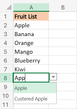
In Excel 365, there is a cool AutoComplete feature for data validation lists. This feature is built-in when using Data Validation for lists in Office 365.

When you are entering data in big lists, you can type the starting letters of what you are looking for in the drop down cell.

The AutoComplete will then find and show you matches from the list. As you type more letters, the options get more specific, and if you delete some letters, it shows more matches.

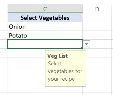
Create a Drop Down List With Message

Want to show a message when someone clicks a drop down cell?

Here is how:

◼ Open the “Data Validation” window.

◼ Click on the “Input Message” tab.

◼ Check the box next to “Show input message when cell is selected.”

◼ In the “Title” and “Input message” boxes, type the message you want to appear (up to 225 characters).

◼ Click “OK” to save the message and close the window.

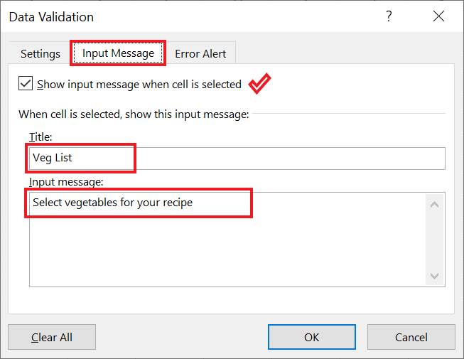
Now, whenever someone clicks the drop down cell, they will see your helpful message!

How to Select All Cells that Have a Drop Down List

Finding cells with drop down lists can be tricky. Here is a quick way to select them all at once:

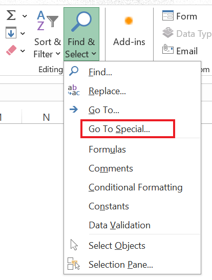
◼ Go to the “Home” tab and click the arrow in the “Find & Select” section.

◼ Choose “Go To Special”.

◼ In the “Go To Special” window, select “Data Validation”.

◼ Choose “All” to select all cells with any data validation rule (including drop down lists).

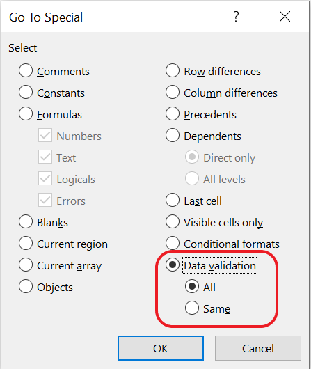
Now you can easily format these cells with a border or background color to make them visually distinct.

Bonus tip: Keep the drop down arrow always visible using another techniques by Jon Acampora.

Attention When Copying Cells With Drop Down Lists in Excel

Be careful when copying and pasting! If you copy a cell without a drop down list over a cell containing a drop down list, the drop down list will be lost. Worse yet, Excel won’t warn you about this happening.

Remember to check your data after copying and pasting, especially when dealing with drop down lists.

Practice Workbook

Conclusion

Excel drop down lists are invaluable tools for improving data entry efficiency, ensuring data accuracy, and enhancing user experience.

By mastering the various creation methods and advanced techniques outlined in this guide, you can streamline your spreadsheet workflow and unlock the full potential of drop down lists in Excel.

Whether you are a beginner looking to get started or an experienced user seeking to optimize your Excel skills, incorporating drop down lists into your spreadsheets will undoubtedly elevate your productivity and organization.

Experiment with different methods, explore additional features, and customize your drop down lists to suit your specific needs, and watch as your Excel proficiency reaches new heights.

Join me on Instagram, YouTube and WhatApp Channel for your daily dose of valuable tips and tricks! Catch insightful videos that will enhance your knowledge and skills. Don’t miss out – follow me now!