Data Brilliance with Excel XLOOKUP Function: Your Ultimate Guide!

Note: Excel XLOOKUP function is exclusively accessible in Microsoft 365’s Excel and Excel for the web. It is not supported in pre-dynamic array versions of Excel (Excel 2019 and earlier) because they do not support array constants. To learn more about how to use Excel for Web for free. Watch 👇 this video

How to Get Microsoft Excel for Free | Free Microsoft Office | Microsoft Office 365

Examples of the Excel XLOOKUP Function

Here are a few examples of using the Excel XLOOKUP function:

Example 1: Basic Usage (Exact Match)

Imagine you have the dataset below, and you wish to fetch the salary for Employee ID 105 (lookup_value). The formula below accomplishes this:

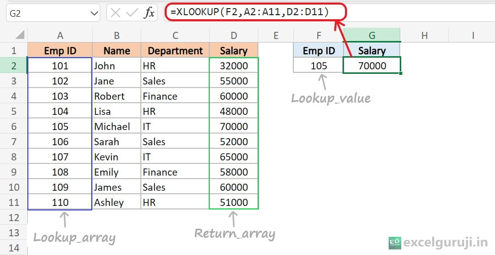
In the formula above, we only used the required arguments of Excel XLOOKUP function. It looks for the Emp ID from A2:A11, finds an exact match, and gives back the matching value from D2 to D11.

A good thing about having the lookup_array and return_array as separate arguments is that now you can also look to the left. VLOOKUP could only find values to the right, but with Excel XLOOKUP Function, that is not a problem anymore.

Now, you will notice in the image below that our lookup array (Emp ID) is on the right side, and the result array (Name) is on the left side. If we want to find the name using the employee ID, we will use the following formula:

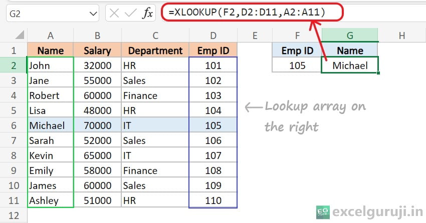
Excel XLOOKUP Function solves a big problem. If you add a new column or change the order of columns, the data will still be right. VLOOKUP might not work correctly in such situations because it often relies on fixed column numbers.

Example 2: Find and Fetch an Entire Record

Using the same data as an example, this time, I don’t just want to retrieve a single piece of information; I want to gather all the records.

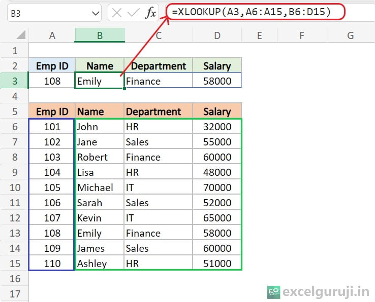
Here is the explanation: =XLOOKUP(A3, A6:A15, B6:D15)

• A3: This is the value you are searching for. The XLOOKUP function is looking for the value in cell A3.
• A6:A15: This is the range in which XLOOKUP searches for the value (A3). It looks in the cells A6 through A15.
• B6:D15: This is the range from which XLOOKUP returns the corresponding value. If a match is found in the range A6:A15, the function will return the corresponding value from the corresponding row in the range B6:D15.

Example 3: If the lookup value is not found

In the image below, you can see that if the lookup value is not found in the lookup array, the formula shows an error.

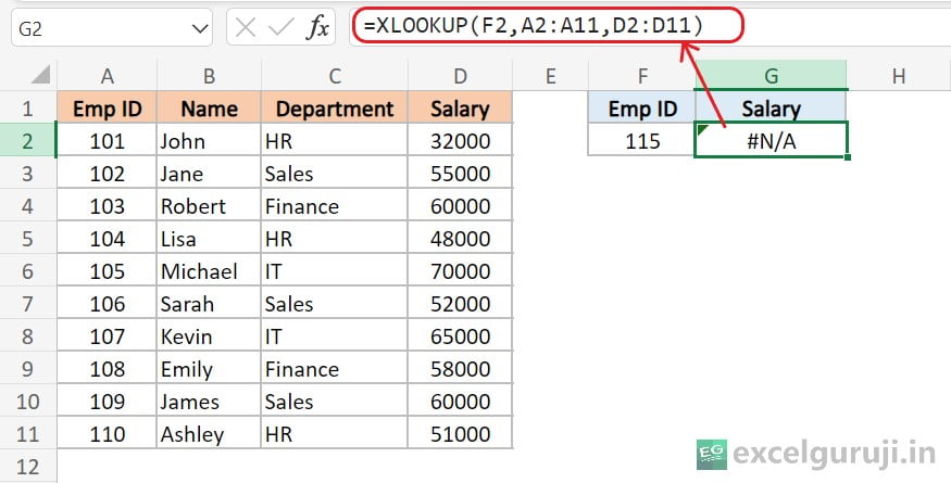
So, if the lookup value is not found, you can utilize the fourth argument, [if_not_found], of the Excel XLOOKUP function to decide what message to write.

The below formula will do this:

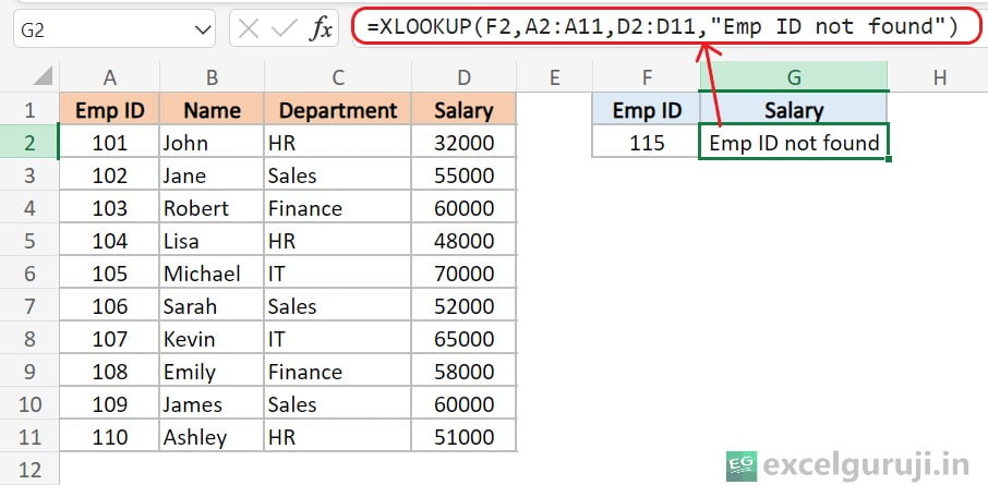
In the example above, we manually specified the desired outcome if no match is found. Alternatively, you can use a cell reference to point to a specific cell or use a formula.

Example 4: Approximate match using XLOOKUP

Let’s explore an example demonstrating the Excel XLOOKUP function in approximate match mode.

XLOOKUP introduces a significant enhancement by offering four match modes, unlike VLOOKUP with two and MATCH with three.

• 0 = exact match (default),
• -1 = exact match or next smallest,
• 1 = exact match or next larger,
• 2 = wildcard match.

You can choose any of these four modes by specifying the corresponding argument to determine how the lookup value should be matched.

Below, you can observe a comprehensive display of various formulas for the match mode, all captured in a single image.

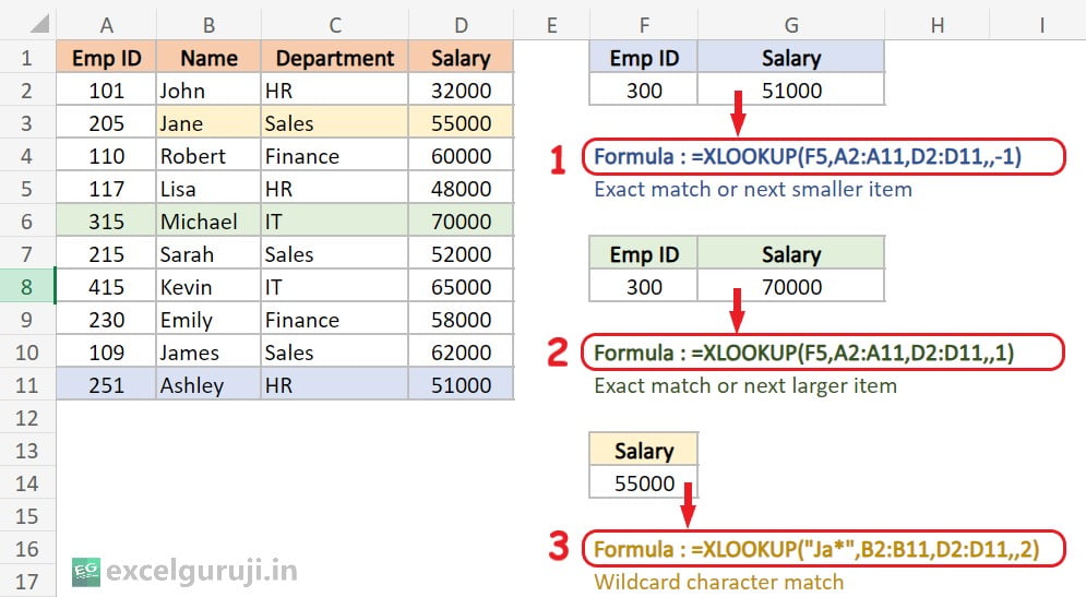
Don’t be confused by seeing so many formulas together; I will explain each one in detail, step by step.

Formula 1 : =XLOOKUP(F2,A2:A11,D2:D11, ,-1)

In the above formula, we omitted the fourth argument [if_not_found], and in the fifth argument [match_mode], we specified -1 for an exact match or the next smaller value.

XLOOKUP formula is searching for the Emp ID ‘300’ in the range of Emp IDs (A2:A11) and, if an exact match is not found, it returns next smaller corresponding salary from the range of Salaries (D2:D11).

In this case, the Emp ID ‘300 is not present in the given dataset. The formula then returns the closest Emp ID less than 300 and provides the corresponding salary, which is 51000 for Employee ID 251.

Formula 2 : =XLOOKUP(F2,A2:A11,D2:D11, ,1)

In the fifth argument [match_mode], we specified 1 for an exact match or the next larger value.

The formula then returns the closest Emp ID larger than 300 and provides the corresponding salary, which is 70000 for Employee ID 315.

Formula 3 : =XLOOKUP(“Ja*”,B2:B11,D2:D11,,2)

In the fifth argument [match_mode], we specified 2 for a Wildcard character match

This formula employs a wildcard character (*) in the lookup value “Ja*”. It searches for names in the range of Names (B2 to B11) that start with “Ja” and may have any characters following. If a match is found, it returns the (first match) corresponding salary from the Salaries column (D2 to D11).

The result is 55000, which is the salary corresponding to the Name “Jane”. The wildcard character (*) enables a partial match based on the specified pattern.

The great advantage is that you no longer have to concern yourself with whether your data is arranged in ascending or descending order. Excel XLOOKUP function seamlessly handles unsorted data.

Example 5: Specifies the search order – first to last or last to first

Normally, XLOOKUP search from the first to the last. If you want it to look from the last to the first, just put -1 in the sixth argument [search_mode] (like in the example below).

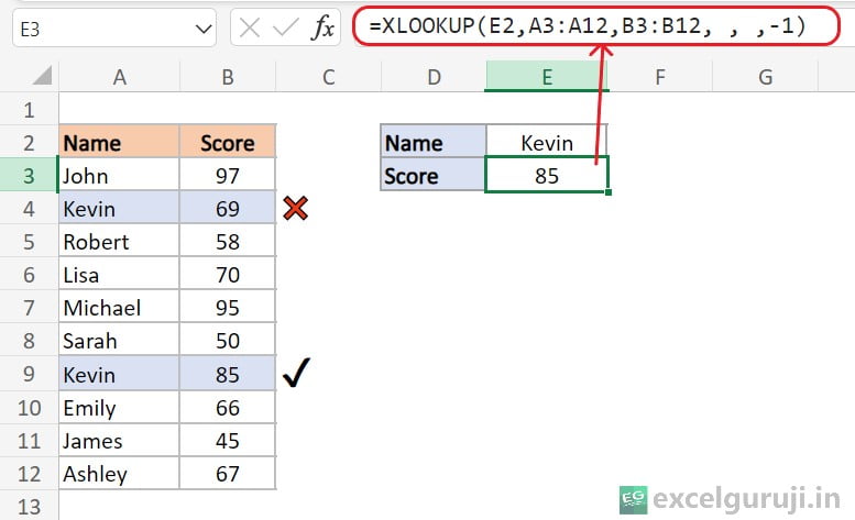
It means that XLOOKUP function should find the value from last to first and match it from the end of the lookup array.

Example 6: Two-Way Lookup with XLOOKUP (Lookup in Both Horizontal and Vertical Directions)

Imagine you have a student report card dataset with names, Math scores, Science scores, and English scores. Now, you want to dynamically find and display the score of a specific subject for a particular student. In this case, we want to find Lisa’s English score, so we will use the following formula:

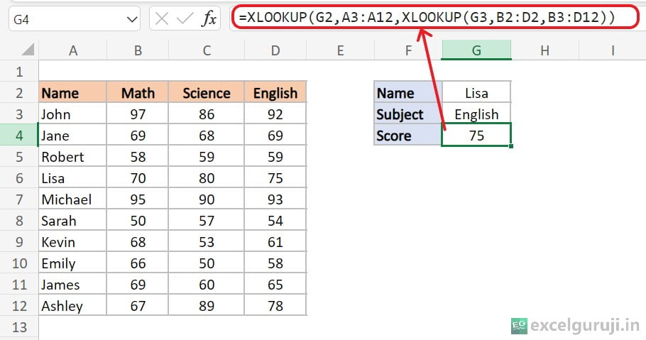
Here is the explanation: =XLOOKUP(G2,A3:A12,XLOOKUP(G3,B2:D2,B3:D12))

This formula uses a Nested XLOOKUP, where first we use it to fetch all the marks of the subject in cell G3

So the result of =XLOOKUP(G3,B2:D2,B3:D12) is {92,69,59,75,93,54,61,58,65,78}, which is an array of English score in this case.

This is used again in the outer XLOOKUP formula as the part that gives back the answer. In this outer XLOOKUP, we look for the student’s name (in cell G2), checking in the range from A3 to A12.

In this case student’s name is Lisa (who is in the fourth position), this outer XLOOKUP formula retrieves the fourth value from the return array, which, in this example, is {92,69,59,75,93,54,61,58,65,78}.

The advantage of using this two-way lookup is that the result doesn’t depend on the student or subject name. If I switch the subject to Math, this XLOOKUP formula would still function correctly and provide the accurate result.

Extra Notes

● If the [if_not_found] argument is omitted, the function returns an #N/A error if no match is found.

● XLOOKUP supports both horizontal and vertical lookup.

● The lookup_array and return_array in XLOOKUP must be the same sizes. If not, XLOOKUP shows an error: #VALUE!

● If XLOOKUP looks at an Excel Table in another file, that file must be open. If not, XLOOKUP shows an error: #REF!

● XLOOKUP can find data on the right or left side of the lookup values.

● XLOOKUP can perform a reverse search (from last to first).

● XLOOKUP can return whole rows or columns, not just one value.