Contents
Excel PMT Function

When to Use the Excel PMT Function in Excel
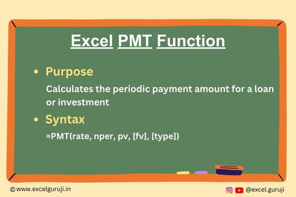
The PMT function1 in Excel is a powerful tool used when dealing with financial calculations, particularly for loans or investments. It helps in calculating the periodic payment for a loan or the investment required to reach a financial goal.
What Excel PMT Function Returns
The Excel PMT function returns the periodic payment amount for a loan or investment, considering a constant interest rate and a fixed period.
Syntax of Excel PMT Function
The syntax of the Excel PMT function is as follows:
=PMT(rate, nper, pv, [fv], [type])
Input Arguments
Here are the input arguments for the Excel PMT function:
● rate: The interest rate for each period.
● nper: The total number of payment periods..
● pv: The present value, or the total amount of the loan or investment.
● [fv]: (Optional) The future value, or a cash balance you want to attain after the last payment. If omitted, it is assumed to be 0.
● [type]: (Optional) The timing of the payment. Use 0 if payments are due at the end of the period, and 1 if payments are due at the beginning. If omitted, it is assumed to be 0.
Examples of the Excel PMT Function
Here are few examples demonstrating the usage of the Excel PMT function:
Example 1: Calculating Loan Payments
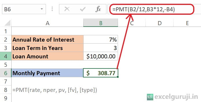
Suppose you have a loan of $10,000 with an annual interest rate of 7%, and you plan to repay it over 3 years (considering a constant interest rate and a fixed period). In cell B6, input the following formula to calculate the monthly payment:

Let’s break down the formula: =PMT(B2/12,B3*12,-B4)
- B2/12: The annual interest rate is in cell B2, which is 7%. To get the monthly interest rate, we divide this by 12 (the number of months in a year). So, B2/12 becomes 7%/12 or 0.0058333 (approximately).
- B3*12: The loan term is in years, and it is given in cell B3 as 3 years. To get the total number of monthly payments, we multiply this by 12. So, B3*12 becomes 36.
- –B4: The loan amount is in cell B4, which is $10,000.00. This value is usually negative in the PMT function to represent an outgoing payment.
When you calculate this, it results in approximately $ 308.77.
Tip: To calculate the overall amount paid throughout the loan term, simply multiply the PMT value obtained by the total number of payment periods (nper).
Example 2: Investment Planning
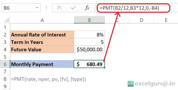
If you aim to save $50,000 for a future project and expect an annual return of 8% over 5 years, you can calculate the monthly savings required using the Excel PMT function. In cell B6, input the following formula:

Let’s break down the formula: =PMT(B2/12,B3*12,0,-B4)
- B2/12: The annual interest rate is in cell B2, which is 8%. To get the monthly interest rate, we divide this by 12 (the number of months in a year). So, B2/12 becomes 8%/12 or approximately 0.0066667.
- B3*12: The term is in years, and it is given in cell B3 as 5 years. To get the total number of monthly payments, we multiply this by 12. So, B3*12 becomes 60.
- 0: This represents the present value, set to 0 in this scenario because you are starting with no initial savings (present value).
- -B4: The future value in cell B4 is $50,000. Although it is considered an incoming payment at the end of the term, by using a negative sign before the cell address, it signifies an outflow of funds from your pocket over a period of 5 years.
When you calculate this, it should indeed result in approximately $680.49. This positive value indicates the monthly savings required to reach a future value of $50,000 over a 5-year period at an 8% annual interest rate.
Note: Here, we use [FV] 4thargument instead of PV 3rd argument, because when saving for a goal, you might set [FV] as the target amount you want to achieve. PMT would then represent the regular savings or investment amount needed to reach that future value. On the other hand, PV might represent an initial investment or loan amount. The choice between using PV or FV depends on the specific financial scenario you are modeling or calculating.
Example 3: Handling Optional Argument
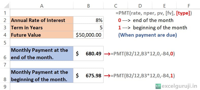
We used the [fv] (4th argument) in the example 2; now, let’s explore how the investment varies by incorporating the [type] (5th argument).
In this example, we will utilize the same parameters as in Example 2.

In the above example, we introduce the [type] parameter, the 5th argument in the PMT function, which allows us to specify when payments are made – either at the beginning or the end of the month.
- =PMT(B2/12, B3*12, 0, -B4, 0)
- The [type] parameter is set to 0, indicating payments are made at the end of the month. If you omit the [type] parameter, the function defaults to 0. This means that, by default, payments are considered to occur at the end of each month.
- =PMT(B2/12, B3*12, 0, -B4, 1)
- The [type] parameter is set to 1, indicating payments are made at the beginning of the month.
Extra Notes
● If the interest rate is less than or equal to -1 or the number of payment periods is 0, you will see a #NUM! error.
● When any of the given values are not numbers, you will get a #VALUE! error.
● When figuring out monthly or quarterly payments, make sure to change annual interest rates or the number of periods into months or quarters.
● To know the total paid over the loan time, just multiply the PMT amount by the number of payments (nper).
● The Excel PMT function gives you the loan amount and interest but doesn’t include extra costs like fees, taxes, or reserve payments.
● If the PMT result is way higher or lower than expected, double-check that you are using the right units for interest rate and number of periods. Make sure to convert annual rates to monthly or quarterly rates, and years to weeks, months, or quarters, as shown in previous examples.
Practice Workbook
There are two sheets in practice file
Download Free Excel File For PracticeConclusion
In conclusion, the Excel PMT function is an indispensable tool for anyone involved in financial planning. Whether you are calculating loan payments, determining required savings, or analyzing investment opportunities, the PMT function provides valuable insights into the financial aspects of your projects.
Remember, practice is key to mastering Excel functions, so don’t hesitate to experiment and apply the PMT function in different financial scenarios. Start utilizing the Excel PMT function today and enhance your financial analysis capabilities in Excel!
Frequently Asked Questions (FAQs)
Q1: Can the Excel PMT function be used for irregular payment intervals?
A1: No, the PMT function is designed for regular payment intervals. For irregular intervals, other financial functions like XNPV or XIRR may be more suitable.
Q2: How does the PMT function handle different compounding frequencies?
A2: The rate and nper should have consistent compounding frequencies. If the payment is monthly, both rate and nper should reflect monthly values.
Q3: Is it necessary to include the optional parameters in the PMT function?
A3: No, the [fv] and [type] parameters are optional. If not needed, you can omit them from the formula.
Q4: Can the PMT function be used for calculating mortgage payments?
A4: Yes, the PMT function is commonly used for calculating mortgage payments, assuming a fixed interest rate and term.
Q5: What does the negative sign in the PMT result signify?
A5: The negative sign indicates that the calculated value is an outgoing payment, such as a loan repayment or an investment contribution.
Click here to download the free Mortgage Calculator Template (With Extra Payment)
Other Related Excel Functions
Excel Mastery: Unveiling the Secrets of the Excel PPMT Function for Precise Principal Payments
Join me on Instagram, YouTube and WhatApp Channel for your daily dose of valuable tips and tricks! Catch insightful videos that will enhance your knowledge and skills. Don’t miss out – follow me now!
1 thought on “Excel PMT Function Mastery: A Comprehensive Guide to Financial Planning”