Contents
Excel FILTER Function
When to Use the Excel FILTER Function in Excel
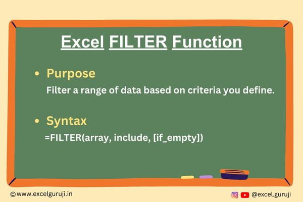
The FILTER function in Excel is a powerful tool for filter specific data from a range based on specified criteria.
It is incredibly handy for managing and analyzing large datasets, helping you quickly retrieve the information you need while leaving out the rest.
What Excel FILTER Function Returns
The Excel FILTER function returns a dynamic array that includes only the rows from a given range that meet the specified conditions. This function is particularly useful when you want to filter data based on one or multiple criteria.
Syntax of Excel FILTER Function
The syntax of the Excel FILTER function is as follows:
=FILTER(array, include, [if_empty])
Input Arguments
Here are the input arguments for the Excel FILTER function:
● array: This is the range of data that you want to filter. It can be a reference to a range of cells, a table, or an array.
● include: This is the array or range of cells where you specify the conditions that the data must meet to be included in the filtered results.
● [if_empty]: This argument is optional. You can use it to specify what should be returned if there are no matching results. If omitted, it will return #CALC! error.
Extra Notes
● Excel FILTER function is exclusively accessible in Microsoft 365’s Excel and Excel for the web. To learn more about how to use Excel for Web for free. Watch 👇 this video
How to Get Microsoft Excel for Free | Free Microsoft Office | Microsoft Office 365
● Make sure the include argument matches the size of the list, or FILTER will not work.
● You can also use multiple criteria to filter the data by providing an array of conditions.
Examples of the Excel FILTER Function
Here are few examples of using the FILTER function in Excel:
Example 1: Basic Usage
Suppose you have a table of sales data in columns A and B. You want to filter the data to show only the rows where the sales value is greater than 1,000. In a new range, enter the following formula:
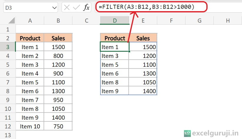
Here is an explanation of the formula: =FILTER(A3:B12, B3:B12 > 1000)
- A3:B12: This is the dataset or range of data you want to filter. In this example, it includes two columns: Product in column A and Sales in column B. The range starts from cell A3 and ends at B12.
- B3:B12 > 1000: This part defines the condition for filtering. It specifies that only rows where the value in column B (Sales) is greater than 1000 should be included in the result.
So, when you enter this formula, it will return a filtered list of rows from the original dataset (A3:B12), where the Sales value in column B is greater than 1000.
Example 2: Using Multiple Criteria
Let’s say you have a list of products in column A, their sales in column B, and you want to filter the products that meet two criteria: the product should be a Laptop, and its sales should be more than 1000. In a new range, enter the following formula:
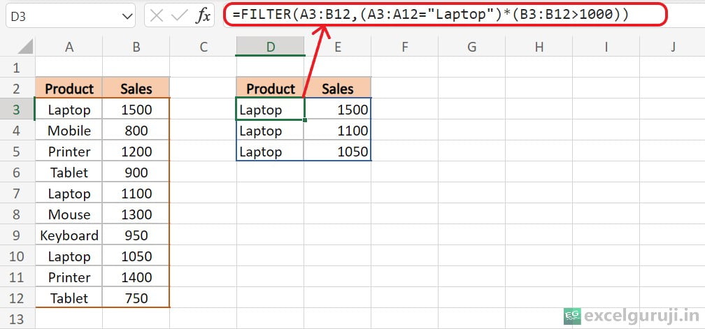
=FILTER(A3:B12,(A3:A12=”Laptop”)*(B3:B12>1000))
- A3:A12=”Laptop” : It selects rows where the corresponding cell in column A (Product) is equal to Laptop.
- B3:B12>1000: It also checks if the corresponding cell in column B (Sales) is greater than 1000.
In other words, it filters the data to show products that are labeled as Laptop and have sales exceeding 1000.
Example 3: Handling Empty Results
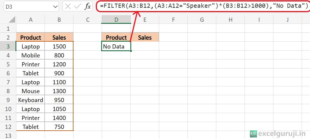
If there are no matching results, the FILTER function will return an error by default. As shown in the formula below, when it doesn’t find a product named “Speaker” anywhere in the range from A3:A12, it gives a #CALC! error because it couldn’t find a matching result.
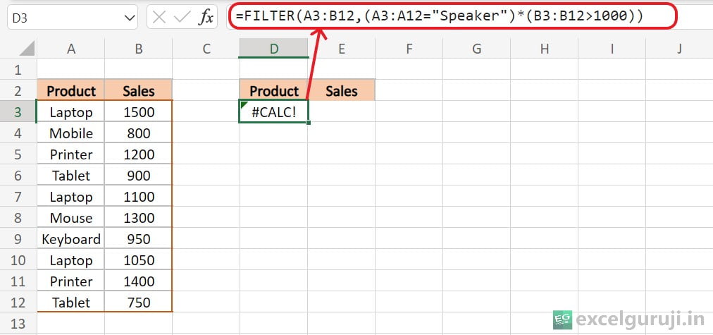
In such cases, you can customize the error using an [if_empty] argument, as demonstrated in the following formula.
Example 4: Dynamic Filtering with Cell References
Using cell references in formulas provides flexibility, ease of maintenance, and reduces the risk of errors, making your spreadsheet more efficient and user-friendly. If you enter a cell reference and later change the value in that cell, your formula will automatically update to reflect the new value.
This allows for dynamic and real-time adjustments without the need to modify the formula itself.
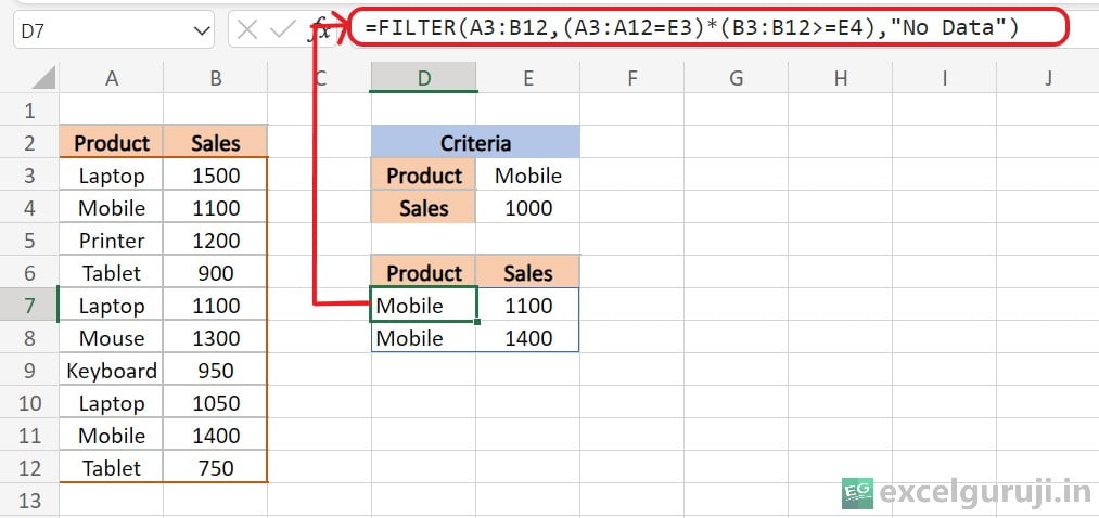
In the image, you can observe how this formula dynamically updates its results as we change the values in cells E3 and E4. This level of flexibility allows for real-time adjustments without the need to alter the formula manually.
Let’s Practice What You have Learned.
Now, it is your turn to try out the Excel FILTER function. You can use the Excel file we have provided to practice and see how it works with sample data.
If you have any questions or if you discover something interesting, please feel free to share your thoughts in the comments. Enjoy learning through hands-on experience!
Conclusion
In conclusion, the Excel FILTER function is a versatile tool that simplifies the process of extracting specific data from a large dataset.
Whether you are working with sales records, inventory information, or any other dataset, the FILTER function can save you time and help you make more informed decisions.
Like any Excel function, mastering FILTER takes practice. Don’t hesitate to experiment with different filtering criteria and explore its various applications in your own projects.
Start using the FILTER function today and take your Excel skills to the next level!
Frequently Asked Questions (FAQs)
Q1: Can the FILTER function be used to filter data based on multiple conditions?
A1: Yes, the Excel FILTER function is capable of filtering data based on single or multiple conditions. You can specify multiple criteria in the include argument.
Q2: What happens if there are no matching results when using the FILTER function?
A2: If there are no matching results, the FILTER function will return an error by default. You can use the [if_empty] argument to customize the output in such cases.
Q3: Can the FILTER function return results in multiple cells?
A3: Yes, the FILTER function can return results in multiple cells if there are multiple matching rows in the filtered data.
Q4: Is the FILTER function case-sensitive?
A4: No, the FILTER function is not case-sensitive by default. It treats text in a case-insensitive manner, so “Laptop” and “LAPTOP” would be considered the same when filtering with the FILTER function.
Q5: What other Excel functions complement the FILTER function for data analysis?
A5: Excel functions like SORT, SUMIFS, COUNTIFS, and AVERAGEIFS can be used in conjunction with the FILTER function to perform advanced data analysis and reporting.
Other Related Excel Functions
Excel CHOOSE Function: A Guide to Efficient Data Selection
Mastering Excel CHOOSECOLS Function: Custom Data Extraction and Analysis
Join me on Instagram, YouTube and WhatApp Channel for your daily dose of valuable tips and tricks! Catch insightful videos that will enhance your knowledge and skills. Don’t miss out – follow