Mastering Excel CHOOSEROWS Function: Select and Extract Rows Like a Pro

Excel CHOOSEROWS Function

When to Use the Excel CHOOSEROWS Function in Excel

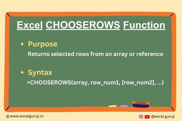
The CHOOSEROWS function in Excel is a powerful tool that allows you to select and extract specific rows from a range of data. This function is particularly useful when you need to filter and work with specific data points or create custom data views based on specific criteria.

What Excel CHOOSEROWS Function Returns

The Excel CHOOSEROWS function returns a new range that consists of the selected rows from the input data range.

Syntax of Excel CHOOSEROWS Function

The correct syntax for the Excel CHOOSEROWS function is as follows:

=CHOOSEROWS(array, row_num1, [row_num2], …)

Input Arguments

Here are the input arguments for the Excel CHOOSEROWS function:

● array: The array represents the source data from which you want to extract rows. It can be a reference to a cell range containing your data or a named range.

● row_num1, [row_num2], …: These are positive integers that indicate which rows you want to select from the data array. You can specify one or more row numbers separated by commas.

Extra Notes

● Excel CHOOSEROWS function is exclusively accessible in Microsoft 365’s Excel and Excel for the web. To learn more about how to use Excel for Web for free. Watch 👇 this video

How to Get Microsoft Excel for Free | Free Microsoft Office | Microsoft Office 365

● If the number you put in the row_num argument is zero or goes beyond the total number of columns in your data, it will give you a #VALUE error.

● The order of the selected rows in the returned range matches the order in which they are specified in the row_num arguments.

Here are few examples of using the Excel CHOOSEROWS function in Excel:

Example 1: Basic Usage

Suppose you have a dataset, and you want to extract specific rows. You can do this using the following formula:

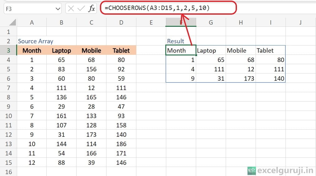
Here’s a breakdown of how it works: =CHOOSEROWS(A3:D15, 1, 2, 5, 10)

• A3:D15: This is the dataset or data range from which you want to extract rows. It consists of 13 rows.
• 1, 2, 5, 10: These are the row numbers you want to extract from the data range.

So, the result of this formula would be a new range that contains only rows 1, 2, 5 and 10 from the original data range A3:D15. The order of the selected rows in the result matches the order in which they are specified in the formula.

You can also provide the row numbers by typing them in different cells. Then, you have the choice to use the cell references for each row number you need, or you can use a range reference for a single row number argument.

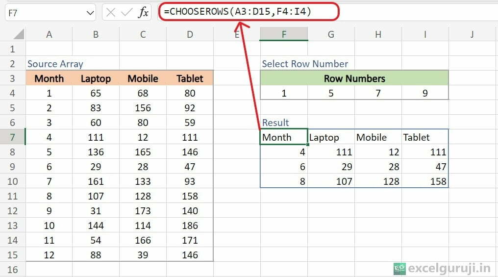
One great thing about this method is that you can easily get different rows just by changing the numbers in those special cells. You don’t have to mess with the formula itself.

Example 2: Extract Rows From the End of an Array

To easily grab the last N rows from a range, use negative numbers for the row numbers. This makes the function count rows starting from the array’s end.

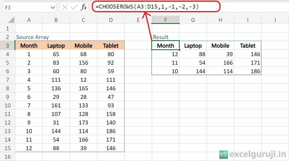
The formula =CHOOSEROWS(A3:D15, 1, -1, -2, -3) in Excel extracts the first row and the last three rows from the end in the dataset defined by the range A3:D15. When using a negative value like -1, -2, -3, it counts rows from the end of the range.

Example 3: Change the Sequence of Rows in an Array.

To turn an array upside down, starting from the top and going down, you can use a combination of Excel functions like CHOOSEROWS, SEQUENCE, and ROWS. For instance:

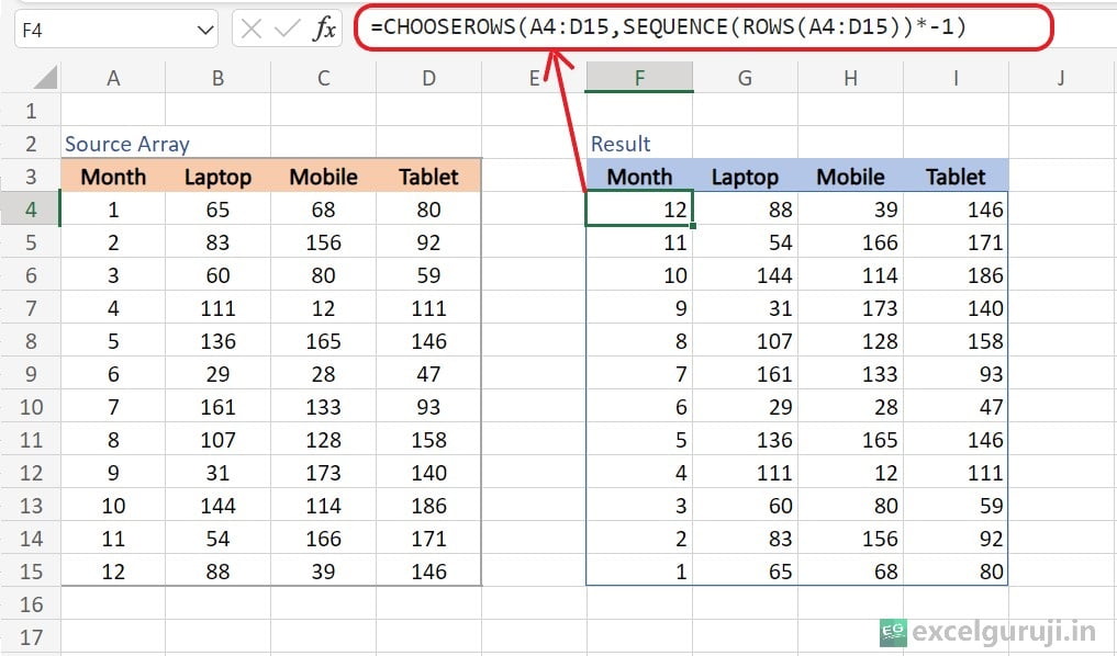
Let’s break it down step by step: =CHOOSEROWS(A4:D15, SEQUENCE(ROWS(A4:D15)) * -1)

• A4:D15: This is a cell range.
• ROWS(A4:D15): This function calculates the number of rows in the specified range A4:D15. In this case, there are 12 rows.
• SEQUENCE(ROWS(A4:D15)): The SEQUENCE function generates an array of sequential numbers. Here, it is generating a sequence of numbers from 1 to 12 (since there are 12 rows in the range A4:D15).
• SEQUENCE(ROWS(A4:D15)) * -1: This part of the formula multiplies each number in the sequence by -1. So, it produces a sequence of numbers from -1 to -12.
• CHOOSEROWS(A4:D15, SEQUENCE(ROWS(A4:D15)) * -1): Excel CHOOSEROWS function is used to choose rows from a given range based on a specified sequence of numbers. In this case, it will choose rows from the range A4:D15 based on the sequence of numbers from -1 to -12.

So, this formula generates a new range of rows from the original range A4:D15, where the order of the rows is reversed. The original data’s rows from A4 to D15 are selected in reverse order, so row 15 is at the top, and row 4 is at the bottom in the resulting range.

Example 4: Extract Only Even Rows

For a straightforward way to isolate even rows from your dataset, use below formula. It simplifies the process, making data analysis more efficient and effective.

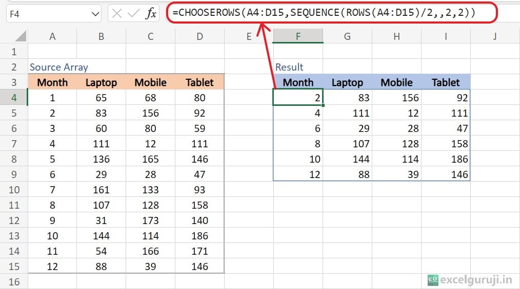
The formula =CHOOSEROWS(A4:D15, SEQUENCE(ROWS(A4:D15)/2, , 2, 2)) in Excel does the following:

• A4:D15: This is the original cell range.
• ROWS(A4:D15): This function calculates the number of rows. There are 12 rows in our case.
• ROWS(A4:D15)/2: Here, we take the number of rows (12) and divide it by 2, resulting in 6. This means we are going to work with the 6 rows of the range A4:D15.
• SEQUENCE(ROWS(A4:D15)/2, , 2, 2): The SEQUENCE function makes a list of numbers in order. In this case, it makes a list of 6 numbers. We don’t need to worry about columns here so we omitted columns argument. It starts with the number 2 and adds 2 more each time. So, it gives us the numbers 2, 4, 6, 8, 10, and 12. These numbers match the even rows in the original data.
• CHOOSEROWS(A4:D15, SEQUENCE(ROWS(A4:D15)/2, , 2, 2)): Excel CHOOSEROWS function is used to choose rows from the range A4:D15 based on the sequence of numbers generated in the previous step (2, 4, 6, 8, 10, 12).

Example 5: Extract Rows From Various Ranges.

If you want to grab specific rows from different ranges that are not next to each other, you can start by combining all the ranges into a single one using the Excel VSTACK function. After that, you can work with the combined range using Excel CHOOSEROWS function.

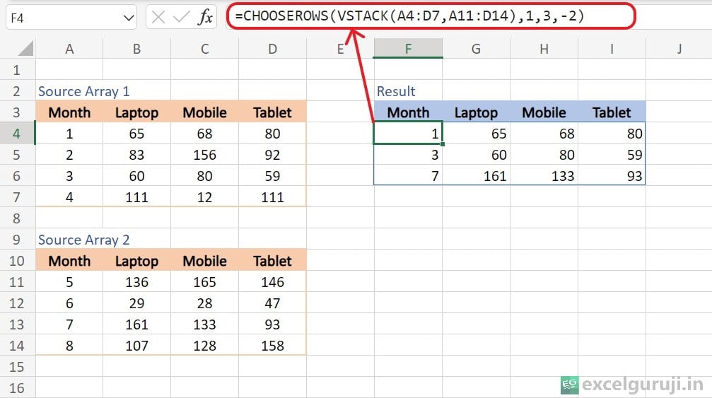
The formula =CHOOSEROWS(VSTACK(A4:D7, A11:D14), 1, 3, -2) in Excel does the following:

VSTACK Function: It combines data from two non-contiguous ranges (A4:D7, A11:D14) into a single continuous range.

CHOOSEROWS Function: It selects and extracts specific rows from the combined range.

Let’s Put Into Practice What We Have Learned.

Let’s try out the Excel CHOOSEROWS function together. You can use the Excel file below to try it out and see how it works. Inside the file, you will find some example data and pre-made CHOOSEROWS formulas to help you get started.

If you have any questions or if you discover something interesting, please share your thoughts in the comments. Have fun learning by doing!

Conclusion

In conclusion, the Excel CHOOSEROWS function is a versatile tool for customizing your data analysis and extraction tasks. Whether you need to filter specific rows, create custom reports, or extract data based on dynamic criteria, Excel CHOOSEROWS function simplifies the process of selecting specific rows to work with.

Just like with any Excel function, practice is key to mastering the Excel CHOOSEROWS function. Experiment with different scenarios and explore its applications in your projects to enhance your Excel proficiency and efficiency.

Frequently Asked Questions (FAQs)

Q1: Can the CHOOSEROWS function select rows from multiple data arrays?

A1: No, Excel CHOOSEROWS function works with a single data array at a time. If you need to select rows from multiple data arrays, you can merge the data using the Excel VSTACK function and then apply the Excel CHOOSEROWS function.

Q2: Can the CHOOSEROWS function reorder the selected columns in the output range?

A2: No, the CHOOSEROWS function returns the selected columns in the same order as they are specified in the row_num arguments.

Q3: What happens if I specify duplicate column numbers in the row_num arguments?

A3: If you specify the same row number more than once in the row_num arguments, the CHOOSEROWS function will indeed duplicate the row in the output range. Each occurrence of the same row number will result in that column being included again in the output range.

Q4: Can the CHOOSEROWS function be used to filter data based on specific conditions?

A4: No, the CHOOSEROWS function is for selecting rows only. If you need to filter data based on conditions, you should use other functions like FILTER or advanced filtering techniques in Excel.

Other Related Excel Functions

Excel CHOOSE Function: A Guide to Efficient Data Selection

Mastering Excel CHOOSECOLS Function: Custom Data Extraction and Analysis

Join me on Instagram, YouTube and WhatApp Channel for your daily dose of valuable tips and tricks! Catch insightful videos that will enhance your knowledge and skills. Don’t miss out – follow me now!