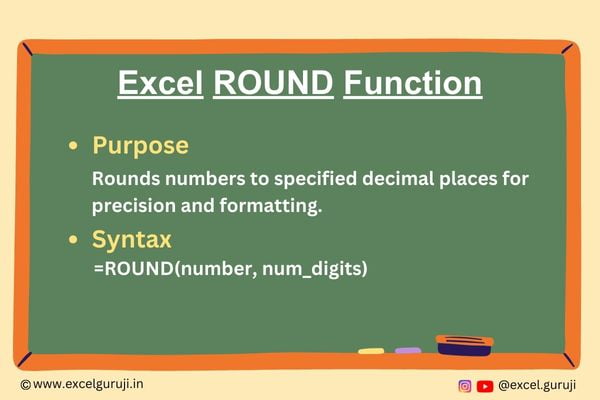
Maximize Precision: Excel ROUND Function for Efficient Number Rounding

Excel ROUND Function

Excel ROUND Function

When to Use the Excel ROUND Function in Excel

Excel ROUND function is used when you need to round a number to a specific number of decimal places. It is particularly useful when dealing with financial data, where precision is essential.

You can also use it to format numbers for presentation purposes, ensuring they are easy to read and understand.

What Excel ROUND Function Returns

Excel ROUND function returns a number rounded to a specified number of decimal places. The result is a numeric value with the desired precision.

Syntax of Excel ROUND Function

The syntax of the Excel ROUND function is as follows:

=ROUND(number, num_digits)

Input Arguments

Here are the input arguments for the Excel ROUND function:

number: The number you want to round. It can be a reference to a cell containing a number, a direct numerical entry, or a formula that evaluates to a numeric value.

num_digits: The number of decimal places to which you want to round the number. This should be a whole number (positive or negative) or a reference to a cell containing such a number.

Extra Notes

● If the specified num_digits is positive, the number is rounded to that many decimal places to the right of the decimal point.

● If num_digits is negative, the number is rounded to the left of the decimal point, effectively rounding to a power of 10.

● If num_digits is non-numeric, the ROUND function returns a #NAME? error.

Examples of the Excel ROUND Function

Here are some examples of using the ROUND function in Excel:

Excel-ROUND-Function-Example

Conclusion

In conclusion, the Excel ROUND function is an essential tool for precision in your numerical calculations and data presentation.

Whether you are working with financial data, mathematical analysis, or simply need to format numbers for readability, the ROUND function can streamline your tasks and improve the clarity of your Excel spreadsheets.

Remember that Excel functions become more powerful as you learn to use them effectively. Don’t hesitate to experiment and discover different applications of the ROUND function in your own projects.

Start using the ROUND function today to enhance your Excel skills and achieve more accurate and readable results.

Frequently Asked Questions (FAQs)

Q1: Can the ROUND function round numbers to the nearest whole number?

A1: Yes, the ROUND function can round numbers to the nearest whole number by specifying 0 as the num_digits argument.

Q2: Can the ROUND function round numbers to a specific number of decimal places to the left of the decimal point?

A2: Yes, the ROUND function can round numbers to a specific number of decimal places to the left of the decimal point by using a negative value for the num_digits argument.

Q3: What happens if the num_digits argument is non-numeric?

A3: If the num_digits argument is non-numeric, the ROUND function returns a #VALUE! error.

Q4: Can I use cell references for both the number and num_digits arguments in the ROUND function?

A4: Yes, you can use cell references for both the number and num_digits arguments in the ROUND function, making it flexible for dynamic calculations.

Q5: What’s the main purpose of the ROUND function in Excel?

A5: The primary purpose of the ROUND function in Excel is to round numbers to a specified number of decimal places for precision and presentation.

Other Related Excel Functions

Mastering Excel SUM Function: Tips and Examples for Efficient Data Calculation (6 Examples)

Mastering Excel SUMIF Function: A Comprehensive Guide for Conditional Summation

Mastering Excel SUMIFS Function: A Comprehensive Guide to Conditional Summing

Join me on Instagram, YouTube and WhatApp Channel for your daily dose of valuable tips and tricks! Catch insightful videos that will enhance your knowledge and skills. Don’t miss out – follow me now!
Excel Online Test 9

Excel-Online-Test-9

Participating in this Excel online test 9 offers more than just an opportunity to showcase your skills; it is a chance for personal growth and self-improvement. Each question you tackle here represents an opportunity to expand your knowledge!

Welcome to your Excel Online Test 9

Total number of questions are 10

Once you have completed the Excel online test, we would greatly appreciate it if you could share your thoughts, feedback, or even your score in the comments section below. Your comments are immensely valuable to us as they guide us in evolving and customizing our content to better suit your needs. So, give it your best effort, and when you’re finished, please don’t forget to leave us a comment.

Your presence in the excelguruji.in community holds immense significance for us, and we sincerely thank you for your active participation!

Ready to elevate your Excel skills? Explore our diverse quiz lineup by clicking below. From basic to advanced, there is a quiz tailored just for you.

Click Here to Explore More Quiz

Your journey to Excel greatness continues. Enjoy the exploration!

Mastering Excel SUMPRODUCT Function: A Comprehensive Guide for Efficient Data Analysis

Excel SUMPRODUCT Function

Excel-SUMPRODUCT-Function

When to Use the Excel SUMPRODUCT Function in Excel

Excel SUMPRODUCT function is a versatile tool that comes in handy when you need to perform calculations on multiple arrays or ranges.

It allows you to multiply corresponding elements in arrays and then sum up those products. This function finds applications in various scenarios, such as calculating weighted averages, scoring systems, and more.

What Excel SUMPRODUCT Function Returns

Excel SUMPRODUCT function returns the sum of the products of corresponding values in the specified arrays or ranges. It is particularly useful for situations where you want to perform complex calculations on multiple sets of data.

Syntax of Excel SUMPRODUCT Function

The syntax of the Excel SUMPRODUCT function is as follows:

=SUMPRODUCT(array1, [array2], [array3], …)

Input Arguments

Here are the input arguments for the Excel SUMPRODUCT function:

array1, array2, array3, …: These are the arrays or ranges you want to multiply and then sum.

Extra Notes

● You can provide up to 255 arrays as arguments.

● The arrays you provide should have the same dimensions. Otherwise Excel SUMPRODUCT returns #VALUE! error.

Non-numeric values in the arrays are treated as zeros in the calculation.

Examples of the Excel SUMPRODUCT Function

Here are four examples of using the SUMPRODUCT function in Excel:

Example 1: Basic Usage

Suppose you have a list of sales quantities in column B and their corresponding prices in column C. You want to calculate the total revenue. You can use the following formula:

Excel SUMPRODUCT Function

Formula: =SUMPRODUCT(B2:B7, C2:C7)

This formula multiplies the Sales Quantity (column B) by the Price (column C) for each product and then sums up the products. When you enter this formula and press Enter, it will give you the total revenue:

  • For Product A: 50 * 652 = 32,600
  • For Product B: 75 * 225 = 16,875
  • For Product C: 80 * 105 = 8,400
  • For Product D: 60 * 79 = 4,740
  • For Product E: 20 * 20 = 400
  • For Product F: 15 * 50 = 750

You will get the total revenue for all products, which is 63,765.

Example 2: Weighted Average

Imagine you have a set of exam scores in column B and their corresponding weights in column C. You want to calculate the weighted average. In cell C7, use the formula:

Excel SUMPRODUCT Function Example 2

Formula: =SUMPRODUCT(B2:B6,C2:C6)

Break down the calculation step by step. Multiply each exam score by its weight:

  • Test 1: 90 * 20% = 18
  • Test 2: 85 * 30% = 25.5
  • Test 3: 78 * 10% = 7.8
  • Test 4: 92 * 20% = 18.4
  • Test 5: 88 * 20% = 17.6

Sum of Products = 18 + 25.5 + 7.8 + 18.4 + 17.6 = 87.3

Example 3: Counting Occurrences

Suppose you have a list of fruits in column A, and you want to count how many times “Apple” appears. You can use the formula:

Excel SUMPRODUCT Function Example 3

Formula: =SUMPRODUCT(–(A1:A5 = “Apple”))

Here’s how the formula works:

(A1:A5 = “Apple”) creates an array of TRUE and FALSE values, where TRUE indicates that “Apple” appears in the corresponding cell, and FALSE indicates it doesn’t. So, it looks like this:

{TRUE, FALSE, TRUE, FALSE, TRUE}

The before the array is a double negation that converts TRUE and FALSE values into 1 and 0, respectively. So, now you have an array of 1 and 0:

{1, 0, 1, 0, 1}

Finally, SUMPRODUCT sums up the values in the array, resulting in the count of occurrences of “Apple”, which is 1 + 0 + 1 + 0 + 1 = 3.

Conclusion

In conclusion, the Excel SUMPRODUCT function is a powerful tool for performing calculations on multiple sets of data. Whether you need to calculate totals, averages, or apply more complex logic, the SUMPRODUCT function can streamline your work and enhance your Excel proficiency.

As with any Excel function, mastering the SUMPRODUCT function takes practice. Don’t hesitate to experiment and explore its various applications in your own projects. Start using the SUMPRODUCT function today to take your Excel skills to the next level!

Frequently Asked Questions (FAQs)

Q1: Can the SUMPRODUCT function handle more than two arrays?

A1: Yes, the SUMPRODUCT function can handle up to 255 arrays as input arguments.

Q2: Can I use the SUMPRODUCT function for non-numeric data?

A2: The SUMPRODUCT function treats non-numeric values as zeros in the calculation, so it’s primarily designed for numeric data.

Q3: What happens if the arrays have different dimensions?

A3: The arrays should have the same dimensions. If the arrays have different dimensions, Excel SUMPRODUCT function returns #VALUE! error.

Q4: Can the SUMPRODUCT function be used for complex conditional calculations?

A4: Yes, you can use logical expressions within the arrays to perform complex conditional calculations using the SUMPRODUCT function.

Q5: Are there other functions in Excel for working with arrays?

A5: Yes, Excel offers a range of array functions, including SUM, AVERAGE, MAX, and MIN, which can be useful for various array-related tasks.

Other Related Excel Functions

SUM Functions

SUMIF Function

SUMIFS Function

Join me on Instagram, YouTube and WhatApp Channel for your daily dose of valuable tips and tricks! Catch insightful videos that will enhance your knowledge and skills. Don’t miss out – follow me now!
Mastering Excel SUMIFS Function: A Comprehensive Guide to Conditional Summing

Excel SUMIFS Function

Excel-SUMIFS-Function

When to Use the Excel SUMIFS Function in Excel

Excel SUMIFS function is used when you want to sum values from a range that meet multiple criteria. It is particularly useful when dealing with large datasets and you need to extract specific subsets of data for analysis or reporting.

Some common scenarios where you might use SUMIFS include sales reports, budget analysis, and expense tracking.

What Excel SUMIFS Function Returns

Excel SUMIFS function returns the sum of values that meet the specified criteria. It allows you to add up numbers from a selected range based on one or more conditions you define.

Syntax of Excel SUMIFS Function

The syntax of the Excel SUMIFS function is as follows:

=SUMIFS(sum_range, criteria_range1, criteria1, [criteria_range2, criteria2], …)

Input Arguments

Here are the input arguments for the Excel SUMIFS function:

sum_range: This is the range of cells that you want to sum when the specified criteria are met. It contains the values you want to add up.

criteria_range1: This is the first range where you set your first condition.

criteria1: This is the condition you want to apply to criteria_range1.

[criteria_range2, criteria2]: You can add more criteria by specifying additional pairs of criteria ranges and conditions. You can have as many criteria pairs as needed.

Extra Notes

● If none of the specified criteria are met in the Excel SUMIFS function, it will return a result of 0.

● You can use wildcards like “*” and “?” in criteria for text matching to match partial text within the criteria_range.

● When using dates in criteria, ensure that the date formats in the criteria match the date formats in the data range to avoid errors.

● Aggregates values based on multiple specified conditions.

● Disregards empty cells or textual data within the sum_range.

● Criteria can be numbers, math stuff, references to cells, words, or special calculations.

● If criteria is a word or a math symbol (like +, -, /, *), it should be in quotation marks.

● Criteria can’t be longer than 255 characters.

● The sum_range and all the criteria_range must have the same size.

Examples of the Excel SUMIFS Function

Let’s go through a few examples to illustrate how to use Excel SUMIFS function effectively:

Example 1: Basic Usage

Suppose you have a sales dataset in which column A contains product names, column B contains sales amounts, and column C contains the region. You want to calculate the total sales for a specific product in a particular region. You can use the following formula:

Excel SUMIFS Function

Let’s break down this formula:

  • B2:B8: This is the range of sales amounts that you want to sum. It covers cells B2 to B8, where your sales data is located.
  • C2:C8: This is the range of regions that you want to filter. It covers cells C2 to C8, where your region names are listed.
  • “Region 1”: This is the criteria for the region. You are specifying that you want to sum sales in “Region 1”.
  • A2:A8: This is the range of product names (Product) that you want to filter. It covers cells A2 to A8, where your product names are listed.
  • “A”: This is the criteria for the product name. You are specifying that you want to sum sales for “Product A.”

Excel SUMIFS function will now go through the Sales, Product, and Region columns, and it will sum up the sales amounts where both the Product is “A” and the Region is “Region 1”.

Example 2: Multiple Criteria

In a similar sales dataset, you may want to calculate the total sales for a specific product in a particular region and within a certain date range. You can use the SUMIFS function with multiple criteria like this:

Excel SUMIFS Function Example 2

Formula: =SUMIFS(B2:B15,C2:C15,”Region 1″,A2:A15,”A”,D2:D15,”>=01-09-2023″,D2:D15,”<=30-09-2023″)

We added additional date criteria to the formula presented in Example 1, which can be described as follows:

  • “>=01/01/2023”: This is the criteria for the starting date of your date range. You are specifying that the date should be greater than or equal to September 1, 2023.
  • “<=12/31/2023”: This is the criteria for the ending date of your date range. You are specifying that the date should be less than or equal to September 30, 2023.

This formula sums the sales amounts where the product name is “A”, the region is “Region 1” and the date falls within the specified range.

Conclusion

In conclusion, the Excel SUMIFS function is a valuable tool for performing conditional summing of data based on multiple criteria.

Whether you are managing financial data, sales records, or any other dataset, Excel SUMIFS function can help you extract and analyze the information you need with precision.

As with any Excel function, practice is key to mastering the SUMIFS function. Experiment with different criteria and conditions in your own projects to become proficient in using this function effectively.

Start using Excel SUMIFS function today and elevate your data analysis capabilities in Excel.

Frequently Asked Questions (FAQs)

Q1: Can I use the SUMIFS function to sum values based on OR conditions?

A1: No, the SUMIFS function is designed for AND conditions. If you need to sum values based on OR conditions, you may consider using the SUMPRODUCT or other functions combined with SUMIFS.

Q2: Are wildcards like “*” and “?” supported in criteria for text matching?

A2: Yes, you can use wildcards like “” (asterisk) and “?” (question mark) in criteria for partial text matching. For example, “apple*” would match any text containing “apple”.

Q3: Can I nest SUMIFS functions for more complex criteria?

A3: Yes, you can nest SUMIFS functions to create more complex criteria by using the result of one SUMIFS function as the sum_range or criteria_range of another SUMIFS function.

Q4: What happens if no values meet the specified criteria in a SUMIFS function?

A4: If no values meet the criteria, the SUMIFS function will return 0.

Q5: Can I use SUMIFS across different worksheets in Excel?

A5: Yes, you can use SUMIFS across different worksheets by referencing the worksheets and cell ranges in your formula.

Other Related Excel Functions

SUM Functions

SUMIF Function

Join me on Instagram, YouTube and WhatApp Channel for your daily dose of valuable tips and tricks! Catch insightful videos that will enhance your knowledge and skills. Don’t miss out – follow me now!

Mastering Excel SUMIF Function: A Comprehensive Guide for Conditional Summation

Excel SUMIF Function

Excel-SUMIF-Function

When to Use the Excel SUMIF Function in Excel

Excel SUMIF function is a powerful tool that allows you to sum values in a range based on specific criteria. It comes in handy when you need to perform calculations on selected data points that meet a certain condition.

Whether you are managing budgets, analyzing sales data, or working with any dataset where conditional summation is required, the SUMIF function can be your go-to solution.

What Excel SUMIF Function Returns

Excel SUMIF function returns the sum of all the numbers in a specified range that meet a given condition or criteria. It provides a way to aggregate data based on user-defined criteria, allowing you to extract meaningful insights from your data.

Syntax of Excel SUMIF Function

The syntax of the Excel SUMIF function is as follows:

=SUMIF(range, criteria, [sum_range])

Input Arguments

Here are the input arguments for the Excel SUMIF function:

range: The range of cells that you want to evaluate against the criteria. This can be a reference to a range or a range specified directly in the formula.

criteria: The condition or criteria that you want to apply to the range. It can be a number, expression, or text that defines what you’re looking for in the data.

sum_range (optional): The range of cells containing the values you want to sum. If this argument is omitted, the SUMIF function will sum the values in the ‘range’ itself.

Extra Notes

● The criteria can include wildcards, comparison operators (>, <, =, etc.), or logical operators (AND, OR) to make your condition more flexible.

● If you want to sum values based on multiple conditions, you can use the SUMIFS function.

● If no cells meet the specified criteria, Excel SUMIF function returns 0.

● You can also use cell references for the range, criteria and sum_range arguments.

Examples of the Excel SUMIF Function

Here are three examples of using Excel SUMIF function:

Example 1: Basic Usage

Suppose you have a list of sales figures in column A, and you want to sum the values that are greater than 3000. In cell A7, use the following formula:

Excel SUMIF Function Example 1 1

The formula will only sum cells that have values greater than 3,000.

Example 2: Summing Values Based on Text Criteria

Let’s say you have a list of products in column A and corresponding sales values in column B. You want to sum the sales for a specific product, “Laptop”. In cell B8, use the formula:

Excel SUMIF Function Example 2

This formula consists of three arguments:

  • A2:A7: This is the range where the criteria (product names) will be checked.
  • “Laptop”: This is the criteria you are looking for, in this case, the product “Laptop”
  • B2:B7: This is the range from which values will be summed if the criteria in column A match “Laptop”.

The result in cell B8 will be the total sales for the product “Laptop”. This means it will sum all the sales values in column B where the corresponding product in column A is “Laptop”.

Conclusion

In conclusion, the Excel SUMIF function is an invaluable tool for conditional summation in Excel. It simplifies data analysis by allowing you to focus on specific subsets of your data that meet certain criteria.

Whether you are managing financial data, tracking inventory, or conducting any data-driven analysis, the SUMIF function empowers you to make informed decisions.

Remember, practice is key to mastering Excel functions. Don’t hesitate to experiment with different criteria and ranges to see how the SUMIF function can work for your specific needs. Start using the SUMIF function today to elevate your Excel skills and streamline your data analysis tasks.

Frequently Asked Questions (FAQs)

Q1: Can the SUMIF function handle multiple conditions simultaneously?

A1: No, the SUMIF function is designed for single-condition summation. If you need to apply multiple conditions, consider using the SUMIFS function.

Q2: Is the SUMIF function case-sensitive when dealing with text criteria?

A2: Yes, the SUMIF function is case-sensitive when it comes to text criteria. “APPLE” and “apple” would be treated as different criteria.

Q3: What happens if no cells meet the specified criteria in the SUMIF function?

A3: In such cases, the SUMIF function returns 0 as the result.

Q4: Can cell references be used for all three arguments of the SUMIF function?

A4: Yes, cell references can be used for the range, criteria and sum_range arguments, providing flexibility in your calculations.

Other Related Excel Functions

SUM Function

SUMIFS Function

Join me on Instagram, YouTube and WhatApp Channel for your daily dose of valuable tips and tricks! Catch insightful videos that will enhance your knowledge and skills. Don’t miss out – follow me now!
Mastering Excel SUM Function: Tips and Examples for Efficient Data Calculation (6 Examples)

Excel SUM Function

Excel-SUM-Function

When to Use the Excel SUM Function in Excel

Excel SUM function is used whenever you need to add up a range of numbers. It comes in handy in various scenarios, such as:

Calculating Total Amounts: You can use the SUM function to find the total sales, expenses, or any other numeric values.

Budgeting and Financial Analysis: When you’re working on a budget or financial analysis, SUM helps you calculate totals quickly.

Statistical Analysis: For statistical analysis, you might need to sum up data points or calculate sums of squares and other statistical measures.

Inventory Management: In inventory management, you can use SUM to keep track of the total stock on hand.

Project Management: When managing projects, SUM can be used to calculate total project costs or hours worked.

What Excel SUM Function Returns

Excel SUM function returns the sum of a range of numbers. It adds up all the values provided as arguments.

Syntax of Excel SUM Function

The syntax of the Excel SUM function is as follows:

=SUM(number1, [number2], [number3], …)

Input Arguments

Here are the input arguments for the Excel SUM function:

number1: This is the first number or range that you want to add.

[number2], [number3], …: These are optional arguments, and you can include multiple numbers or ranges to add.

Extra Notes

● When you use SUM, it conveniently skips over empty cells and those with text, focusing only on numeric values.

● The SUM function can handle ranges with both positive and negative numbers. It will correctly calculate the net sum.

● Keep in mind that if there are any errors within the arguments you provide, the SUM function will also return an error.

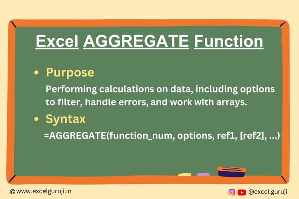
● If you need to sum numbers while ignoring any errors, consider using the AGGREGATE function.

● SUM is quite accommodating; it can handle as many as 255 different arguments in total.

● You have flexibility when it comes to supplying arguments; they can take the form of constants, ranges, named ranges, or cell references.

Examples of the Excel SUM Function

Let’s dive into a few examples of using the Excel SUM function:

Example 1: Basic Usage

Suppose you have a list of sales figures in cells A1 to A5, and you want to find the total sales. In cell A6, you can use the following formula:

Excel-SUM-Function-Example-1

This formula will add up all the values in the range A1 to A5 and display the total in cell A6.

Example 2: Adding Multiple Ranges

In more complex scenarios, you might have sales data in different columns. For instance, you have sales in columns A and C. In this case, you can use the SUM function as follows:

Excel-SUM-Function-Example-2

This formula adds up the values in both ranges and provides the total.

Example 3: Sum Non-contiguous Cells

In Excel, you can also utilize the SUM function to calculate the total of cells that are not positioned next to each other. Non-contiguous, in this context, refers to cells that are not adjacent to one another.

Excel SUM Function Example 3

This formula adds up the values in both ranges and provides the total.

Example 4: Sum Entire Column

In Excel, you have the option to utilize the SUM function to sum up an entire column. This offers the benefit that when you incorporate fresh data into a column, there is no need to redefine a new range.

Excel-SUM-Function-Example-4

Additionally, it’s worth noting that you can employ the SUM function to calculate the total of an entire row as well. For instance, using the formula =SUM(2:2) will add up all the values in the 2nd row.

Example 5: AutoSum

To rapidly calculate the sum of a column or row of numbers, you can either utilize AutoSum or simply press ALT + = (Shortcut).

First, choose the cell located just below the column of numbers or adjacent to the row of numbers that you wish to sum. Then, on the Home tab, within the Editing group, select AutoSum (or use the shortcut ALT + =).

Excel-SUM-Function-Example-51

Ensure there are no gaps with empty cells in between when totaling, as AutoSum will extend the selected range as long as all cells are filled.

Excel-SUM-Function-Example-5

Finally, press the Enter key to get the total.

AutoSum can also be employed to swiftly generate both a total row and a total column. For example, select the range B2:F7 below.

Excel SUM Function Example 52

Now Just click on AutoSum or use the shortcut ALT + =.

Excel automatically adds 10 SUM functions! It’s a simple yet remarkable trick.

Excel-SUM-Function-Example-53

Example 6: Sum Range with Errors

If there’s an error within your cell range and you want to calculate the total, you have two options: you can utilize the AGGREGATE function, or you can achieve the total by employing the IFERROR function, as demonstrated below.

Excel-SUM-Function-Example-6

To do this, you’ll need to utilize an array formula. Apply the array formula by entering the regular formula “=SUM(IFERROR(A1:A10,0))” and then simultaneously pressing Ctrl + Shift + Enter.

Conclusion

In conclusion, the Excel SUM function is a powerful tool for performing addition operations on numeric data in Excel. Whether you are dealing with financial data, statistical analysis, or simple calculations, SUM simplifies the process and ensures accuracy.

Mastering Excel functions like SUM is essential for anyone working with data in Excel. As you gain experience, you will discover more advanced uses and creative ways to leverage this function in your projects. Start using the SUM function today and enhance your Excel skills for better data analysis and management.

Frequently Asked Questions (FAQs)

Q1: Can the SUM function be used for non-numeric values?

A1: No, the SUM function is designed exclusively for adding numeric values. It will ignore any non-numeric cells.

Q2: Can I use the SUM function with conditional criteria?

A2: Yes, you can use the SUM function in combination with other functions like SUMIF or SUMIFS to perform conditional sums based on criteria.

Q3: Is there a limit to the number of arguments the SUM function can accept?

A3: Excel allows you to provide up to 255 arguments to the SUM function.

Q4: Can I use the SUM function with date values?

A4: Yes, you can use the SUM function with date values, and it will add up date values just like numeric values. However, the result may be a date value that needs to be formatted accordingly.

Other Related Excel Functions

SUMIF Function

SUMIFS Function

Join me on Instagram, YouTube and WhatApp Channel for your daily dose of valuable tips and tricks! Catch insightful videos that will enhance your knowledge and skills. Don’t miss out – follow me now!
Excel Online Test 8

Excel-Online-Test-8

Taking this Excel online test is about more than just demonstrating your skills; it is an opportunity for personal growth and self-improvement. Every question you encounter here is a chance to expand your knowledge!

Welcome to your Excel Online Test 8

Total number of questions are 15

After you have completed Excel online test, we’d love it if you could share your thoughts, feedback, or even your score in the comments below. Your comments mean the world to us because they help us evolve and tailor our content to meet your needs. So, give it your all, and when you have finished, please remember to drop us a comment.

Your presence in the excelguruji.in community means the world to us, and we are sincerely grateful for your participation!

Hungry for more Excel challenges? Dive into our quiz collection by clicking below. Each quiz is a stepping stone in your journey to Excel expertise.

Click Here to Explore More Quiz

Excel in every quiz, and let the knowledge flow!

Excel IFERROR Function: Error Handling Made Easy | Tips & Examples

Excel IFERROR Function

Excel-IFERROR-Function

When to Use the Excel IFERROR Function in Excel

Excel IFERROR function is a powerful tool to handle errors and improve the reliability of your Excel formulas. It is used when you want to control how Excel responds to errors that may occur within a formula.

Whether you are working with complex calculations, importing data, or manipulating spreadsheets, the IFERROR function can help ensure your Excel workbooks are error-free.

What Excel IFERROR Function Returns

Excel IFERROR function returns a specified value if a formula or expression results in an error. If there is no error, it returns the result of the formula or expression itself.

This function is particularly useful for preventing error messages from appearing in your worksheets and replacing them with custom messages or values.

Syntax of Excel IFERROR Function

The syntax of the Excel IFERROR function is as follows:

=IFERROR(value, value_if_error)

Input Arguments

Here are the input arguments for the Excel IFERROR function:

value: This is the expression or formula that you want to evaluate for errors. It can be any valid Excel formula.

value_if_error: This is the value or message that you want the function to return if the ‘value’ argument results in an error. It can be a text string, a numeric value, another formula, or even a cell reference.

Extra Notes

● Excel IFERROR function is particularly useful when dealing with functions like VLOOKUP or INDEX-MATCH, which can result in errors if the specified lookup value is not found. Instead of displaying an error message, you can use IFERROR to replace it with a user-friendly message or value.

● You can nest the IFERROR function within other Excel functions to create more advanced error-handling mechanisms. For example, you can use it within an IF statement to perform different actions based on whether an error occurs.

● While IFERROR is excellent for handling errors within individual cells or formulas, it is also essential to audit your entire worksheet for errors regularly. Excel provides auditing tools like the “Error Checking” feature to help you identify and correct errors on a broader scale.

● Remember that Excel IFERROR function only handles errors related to calculation or formula evaluation. It won’t address errors related to data validation or input errors in your worksheets.

Examples of the Excel IFERROR Function

Let’s explore a few examples to see how the IFERROR function works in Excel.

Example 1: Handling Error

You have a column of numbers in Excel, and you want to calculate the reciprocal of each of those numbers. However, you want to ensure that if you encounter a situation where you are dividing by zero (which is mathematically undefined and would result in an error), Excel doesn’t display an error message but instead shows a custom message like “N/A” (which stands for “Not Available”).

Excel IFERROR Function Example 1

To achieve this, you can use the Excel IFERROR function. Here is the formula used:

Excel-IFERROR-Function-Example-1-1

So, using this formula ensures that you won’t encounter error messages due to division by zero in your Excel worksheet, making it more user-friendly and preventing potential confusion when dealing with mathematical operations.

Example 2: Custom Error Messages

Assuming you have a list of products and their corresponding prices in an Excel table, you want to look up the price of a specific product using VLOOKUP. If the product exists, you want to display the price, and if it doesn’t exist, you want to show “Not Found”.

Excel-IFERROR-Function-Example-2

In this case, the VLOOKUP function displays an error because ‘Mango’ is not available in the product table. To handle such errors and show custom error messages, you can use the IFERROR function.

Excel-IFERROR-Function-Example-21

Conclusion

In conclusion, the Excel IFERROR function is a valuable tool for error handling and data validation. It allows you to control how Excel responds to errors, providing a more user-friendly experience for anyone using your spreadsheets.

By using IFERROR, you can make your Excel workbooks more robust and user-friendly, reducing the likelihood of error messages and ensuring that your data and calculations are more reliable.

Frequently Asked Questions (FAQs)

Q1: Can the IFERROR function handle multiple types of errors?

A1: Yes, the IFERROR function can handle various types of errors that may occur in Excel formulas, including #DIV/0!, #VALUE!, #N/A, and more.

Q2: Can I nest IFERROR functions to handle different error types differently?

A2: Yes, you can nest IFERROR functions to create more complex error-handling logic based on different error conditions.

Q3: Can the IFERROR function replace errors with specific values?

A3: Yes, you can specify any value, including text strings, numbers, or even other formulas, as the value_if_error argument to replace errors with custom values.

Q4: What other Excel functions work well with IFERROR for error handling?

A4: Functions like ISERROR, IFNA, and ISNA can complement the IFERROR function for more advanced error handling and analysis in Excel.”

Other Related Excel Functions

IF Function

IFS Function

Join me on Instagram, YouTube and WhatApp Channel for your daily dose of valuable tips and tricks! Catch insightful videos that will enhance your knowledge and skills. Don’t miss out – follow me now!
Mastering Excel IFS Function: Simplify Conditional Logic in Excel

Excel IFS Function

Excel-IFS-Function

When to Use the Excel IFS Function in Excel

Excel IFS function is a powerful tool used to perform multiple conditional checks and return different values based on the first condition that evaluates to true.

It simplifies complex nested IF statements and makes your Excel formulas more concise and easier to read.

What Excel IFS Function Returns

Excel IFS function returns a value based on the first condition that is met. It allows you to specify multiple conditions and corresponding values to return when those conditions are true. If none of the conditions are met, you can optionally specify a default value to return.

Syntax of Excel IFS Function

The syntax of the Excel IFS function is as follows:

=IFS(logical_test1, value_if_true1, [logical_test2, value_if_true2], ……)

Input Arguments

Here are the input arguments for the Excel IFS function:

logical_test1, logical_test2, ….: These are the conditions you want to evaluate. Each logical_test should be a statement that can be either true or false.

value_if_true1, value_if_true2, ….: These are the values you want to return when the corresponding logical_test is true.

value_if_false (optional): This is the value you want to return if none of the conditions are true. If omitted and no conditions are met, the function returns a #N/A error.

Extra Notes

● Excel IFS function is available in versions 2019, Microsoft 365, and Excel Online. If you are using an older version of Excel, you may need to use alternative methods, such as nested IF statements, to achieve similar results.

● You can include up to 127 pairs of logical tests and corresponding values with the Excel IFS function. This flexibility allows you to handle a wide range of conditions in a single formula.

● The logical tests in Excel IFS function are evaluated in the order you provide them. Once a true condition is found, the corresponding value is returned, and the function exits, ignoring the remaining conditions.

● If two or more logical tests are true, only the value associated with the first true condition encountered is returned. It is important to order your conditions appropriately to ensure the desired outcome.

● You can use various comparison operators in your logical tests, such as <, >, <=, >=, =, and <> (not equal to). These operators allow you to create precise conditions for different scenarios.

Examples of the Excel IFS Function

Here are a few examples to illustrate how Excel IFS function can be used in Excel:

Example 1: Basic Usage

Suppose you have a list of scores in column B, and you want to assign grades based on those scores. You can use the IFS function like this:

Excel-IFS-Function-Example-1

This formula will return the corresponding grade based on the score

Example 2: Employee Evaluation

Suppose have a team of employees, and you want to evaluate their performance based on three criteria: productivity, teamwork and communication skills. You want to assign performance ratings to each employee based on these criteria.

Here’s the formula and how it works:

Excel-IFS-Function-Example-2

=IFS((A1+B1+C1)/3>=90, “Outstanding”, (A1+B1+C1)/3>=80, “Excellent”, (A1+B1+C1)/3>=70, “Good”, (A1+B1+C1)/3>=60, “Needs Improvement”, TRUE, “Poor”)

Now, let’s break down how the formula assigns performance ratings:

(A1+B1+C1)/3>=90: This condition calculates the average of the three performance scores (productivity, teamwork, and communication) by adding them up and dividing by 3. If the resulting average score is equal to or greater than 90, it means the employee’s performance is outstanding, and “Outstanding” is assigned as the performance rating.

(A1+B1+C1)/3>=80: If the average score falls between 80 and 89 (inclusive), it indicates excellent performance, and “Excellent” is assigned as the performance rating.

(A1+B1+C1)/3>=70: If the average score falls between 70 and 79 (inclusive), it indicates good performance, and “Good” is assigned as the performance rating.

(A1+B1+C1)/3>=60: If the average score falls between 60 and 69 (inclusive), it suggests that the employee’s performance needs improvement, and “Needs Improvement” is assigned as the rating.

TRUE: This serves as the default condition. If none of the previous conditions are met, it means the average score is below 60, which indicates poor performance. Therefore, “Poor” is assigned as the performance rating.

By using the IFS function in this manner, you can effectively evaluate employee performance based on multiple criteria and provide clear performance ratings, which can be valuable for performance reviews, goal setting, and career development discussions.

Conclusion

In conclusion, the Excel IFS function is a versatile and efficient way to handle multiple conditional statements in your Excel spreadsheets.

It simplifies complex logic and makes your formulas more readable. Whether you are grading students, analyzing data, or categorizing items, the IFS function can streamline your Excel tasks and improve your productivity.

As with any Excel function, practice is key to mastering the IFS function. Experiment with different conditions and values in your own projects to fully harness its capabilities. Start using the IFS function today and take your Excel skills to the next level!

Frequently Asked Questions (FAQs)

Q1: Can I use multiple logical tests with the IFS function?

A1: Yes, you can use multiple logical tests with the IFS function. Simply provide pairs of logical tests and corresponding values to return.

Q2: What happens if none of the conditions in the IFS function are met?

A2: If none of the conditions are met and you haven’t provided a value_if_false argument, the function will return a #N/A error.

Q3: Can I use the IFS function to handle both numeric and text conditions in the same formula?

A3: Yes, you can use both numeric and text conditions in the same IFS formula. Just ensure that each condition is paired with the appropriate value to return.

Other Related Excel Functions

IF Function

Join me on Instagram, YouTube and WhatApp Channel for your daily dose of valuable tips and tricks! Catch insightful videos that will enhance your knowledge and skills. Don’t miss out – follow me now!
Excel IF Function: Mastering Conditional Logic in Spreadsheets

Excel IF Function

Excel-IF-Function

When to Use the Excel IF Function in Excel

Excel IF function is used when you want to perform different calculations or actions based on whether a specified condition is true or false. It is commonly used in scenarios where you need to make comparisons, apply different formulas, or display specific results depending on the data in your worksheet.

What Excel IF Function Returns

Excel IF function returns one value if a specified condition is true and another value if the condition is false. This makes it an excellent choice for creating dynamic and responsive spreadsheets.

Syntax of Excel IF Function

The syntax of the Excel IF function is as follows:

=IF(logical_test, [value_if_true], [value_if_false])

Input Arguments

Here are the input arguments for the Excel IF function:

logical_test: This is the condition you want to evaluate. It can be a logical expression, a comparison, or any statement that results in either true or false.

value_if_true: This is the value or formula to be returned if the logical_test is true.

value_if_false: This is the value or formula to be returned if the logical_test is false.

Extra Notes

● You can nest multiple IF functions together to handle more complex conditions and create multiple outcomes.

● Excel IF function is not case-sensitive, meaning it treats uppercase and lowercase text as the same when evaluating conditions.

● You can use a wide range of logical expressions and comparisons within the logical_test argument, providing flexibility in your conditions.

● If you omit the value_if_false argument, Excel will return 0, if the condition is false.

● It is important to enclose the text in quotation marks, like this: “Text”. However, there is one exception to this rule – when you use TRUE or FALSE, Excel automatically recognizes and interprets them without the need for quotes.

Examples of the Excel IF Function

Here are a few examples to illustrate how the IF function can be used in Excel:

Example 1: Basic Usage

Suppose you have a list of scores in column B, and you want to categorize each score as Pass if it is greater than or equal to 50 and Fail if it is less than 50. You can use the following formula in column C:

Excel-IF-Function-Example-1

Example 2: Nested IF Statements

You can also nest IF statements to create more complex conditions. For instance, you want to categorize scores as High, Medium or Low based on different score ranges. You can use the following nested IF formula:

Excel-IF-Function-Example-2

So, in summary, this formula categorizes the value in cell B2 into one of three categories: High, Medium or Low based on the specified conditions. If the value is 90 or higher, it is High. If it is between 70 and 89, it is Medium. If it is less than 70, it is Low.

Example 3: IF function with AND & OR Function

In this third example, we are about to explore the versatility of the Excel IF function by combining it with both the AND and OR functions.

If you are already comfortable with these concepts, feel free to dive right in. However, if you would like to see how we have previously applied the IF function with the OR and AND functions, we recommend checking out our earlier blog posts.

Mastering the Excel AND Function: A Comprehensive Guide for Effective Spreadsheet Logic

  • In our earlier post, we covered the usage of the IF function with the AND function, highlighting its utility in handling complex conditions.

Excel OR Function: Simplify Decision-Making with Multiple Conditions

  • In this post, we demonstrated how to use the IF function in conjunction with the OR function, allowing you to create conditional logic with multiple options.

Conclusion

In conclusion, the Excel IF function is a powerful tool that allows you to make decisions and perform actions based on specific conditions in your Excel spreadsheets. Whether you need to categorize data, calculate values, or automate tasks, the IF function can simplify your work and make your spreadsheets more dynamic.

Remember that mastering Excel functions, including the IF function, takes practice. Don’t hesitate to experiment and explore different applications of the IF function in your own projects. Start using the IF function today and take your Excel skills to the next level!

Frequently Asked Questions (FAQs)

Q1: Can the IF function handle more than one condition?

A1: Yes, you can nest multiple IF functions to handle multiple conditions in a single formula.

Q2: Are there any limitations to the logical_test argument?

A2: The logical_test argument can include a wide range of logical expressions, comparisons, or functions, making it highly flexible.

Q3: Can the IF function be used with text values?

A3: Absolutely! The IF function can work with both numerical and text values, allowing you to create dynamic text outputs based on conditions.

Q4: Is it possible to have more than two outcomes with the IF function?

A4: Yes, by nesting multiple IF functions, you can create complex conditions with more than two possible outcomes.

Join me on Instagram, YouTube and WhatApp Channel for your daily dose of valuable tips and tricks! Catch insightful videos that will enhance your knowledge and skills. Don’t miss out – follow me now!