Excel Guruji

Excel PROPER Function

When to Use the PROPER Function in Excel

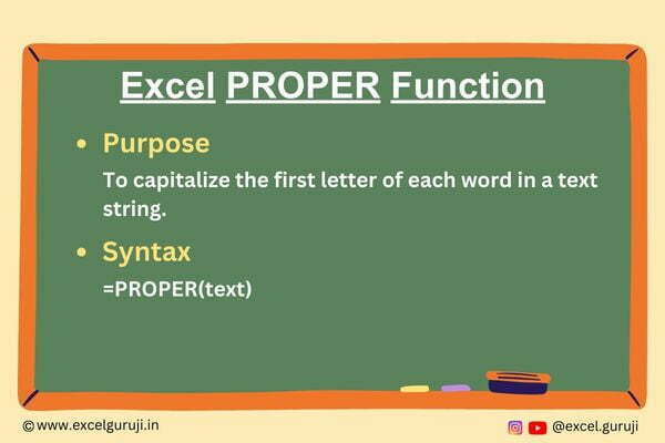
The PROPER function in Excel comes to the rescue when you need to capitalize the first letter of each word in a text string. It finds its utility in scenarios involving data presentation, report generation, or enhancing the visual appeal of your content.

What Excel PROPER Function Returns

The Excel PROPER function is all about capitalization. It transforms a text string into a new one where the first letter of every word is capitalized, while the rest of the letters are converted to lowercase.

Syntax of Excel PROPER Function

The syntax of the Excel PROPER function is as follows:

=PROPER(text)

Input Arguments

Here are the input arguments for the Excel PROPER function:

👉 text: This can be a reference to a cell containing the text, a direct text entry enclosed in quotation marks, or even a formula that evaluates to a text string.

Extra Notes

👉 The PROPER function doesn’t handle acronyms well; it will capitalize every letter in an acronym, which might not be the desired outcome.

👉 Words separated by non-alphabetic characters, such as hyphens or underscores, are also considered as separate words.

👉Words in all uppercase are transformed to title case, where only the first letter is capitalized.

Common Mistakes to Avoid

👉 Neglecting to enclose text entries in quotation marks: If you’re working with a direct text entry, make sure to enclose it in double quotation marks.

👉 Overlooking the impact of special characters: Keep in mind that words separated by non-alphabetic characters will also be capitalized.

👉 Applying the PROPER function to acronyms or all uppercase text unintentionally: Be cautious when using the PROPER function with acronyms or all uppercase text, as it will change the case of every letter.

Tips For Optimal Usage

To maximize the benefits of the Excel PROPER function, consider these tips:

👉 Combine PROPER with other text functions like CONCATENATE or SUBSTITUTE to create complex text transformations.

👉 Use PROPER to clean up data before presentations or when generating reports to ensure a consistent and professional look.

👉 Always review the outcome to verify that the capitalization aligns with your expectations.

Examples of the PROPER Function in Excel

Here are a few instances demonstrating the usage of the PROPER function in Excel:

Example 1: Basic Usage

Assume you have the text “excel functions are powerful” in cell A1. You want to capitalize the first letter of each word. Place the following formula in cell B1:

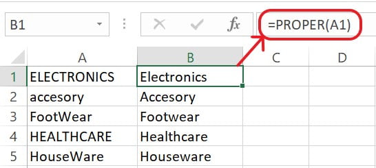
Example 2: Handling Mixed Cases

You have a list of product names in column A, but some of them are in all uppercase, while others are in lowercase. You wish to standardize the capitalization. In cell B2, use this formula:

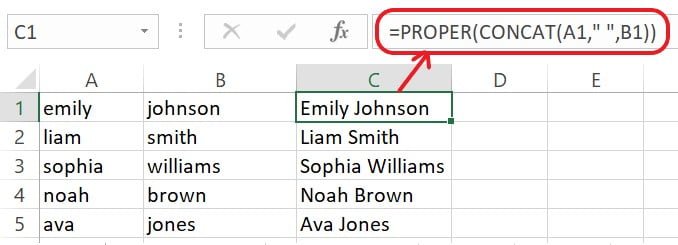
Example 3: Using PROPER with CONCATENATE

Suppose you have two columns, one containing first names and the other containing last names, and you want to create a column with properly formatted full names. Use the following formula

Alternatively, you can use the ampersand “&” operator for concatenation: Like =PROPER(A1&” “&B1)

Conclusion

In summary, the Excel PROPER function is an essential tool for achieving consistent and polished text capitalization. Whether you are creating reports, formatting data, or refining content, the PROPER function simplifies the process and enhances the visual quality of your work.

Remember, becoming proficient in Excel functions takes practice. So, don’t hesitate to experiment with the PROPER function in various scenarios. Start utilizing PROPER today to elevate the presentation of your Excel data.

Frequently Asked Questions (FAQs)

Q1: Does the PROPER function affect acronyms?

A1: Yes, the PROPER function capitalizes every letter in an acronym, which might not be desired. Be cautious when working with acronyms.

Q2: Can I use the PROPER function for capitalizing the entire text?

A2: While you can use PROPER for this purpose, it’s better suited for capitalizing only the first letter of each word. For all uppercase transformations, you can use UPPER functions.

Q3: Does the PROPER function work with special characters?

A3: Yes, the PROPER function considers words separated by non-alphabetic characters as separate words and capitalizes them accordingly.

Q4: Can I use PROPER to capitalize just the first letter of a text?

A4: Absolutely! PROPER is specifically designed to capitalize the first letter of each word in a text string.

Q5: Can the PROPER function handle names with apostrophes?

A5: Yes, the PROPER function handles names with apostrophes correctly, capitalizing the letter after the apostrophe if it’s the first letter of a word.”

Other Related Excel Functions

LEFT Function

RIGHT Function

MID Function

LEN Function

UPPER Function

LOWER Function

Join me on Instagram and YouTube for your daily dose of valuable tips and tricks! Catch insightful videos that will enhance your knowledge and skills. Don’t miss out – follow me now!

Excel LOWER Function

When to Use the LOWER Function in Excel

When it comes to transforming and manipulating text data in Excel, functions like LOWER can be your secret weapon. If you have ever needed to convert text to lowercase, the Excel LOWER function is here to streamline the process and enhance your data processing capabilities.

What Excel LOWER Function Returns

The LOWER function in Excel is your go-to tool when you want to convert uppercase or mixed-case text to lowercase. It is a handy function that can help you to ensure consistency in your data, facilitate comparisons, and prepare text for various types of analysis.

Syntax of Excel LOWER Function

The syntax of the Excel LOWER function is elegantly simple:

=LOWER(text)

Input Arguments

Here are the input arguments for the Excel LOWER function:

👉 text: This is the text you want to convert to lowercase. It can be a reference to a cell containing the text, a direct text entry enclosed in quotation marks, or a formula that evaluates to a text string.

Extra Notes

👉 The LOWER function has no effect on text that is already in lowercase. It only converts uppercase and mixed-case text to lowercase.

👉 The LOWER function affects only alphabetical characters within a text string. Non-alphabetical characters remain unchanged.

👉 If you encounter non-alphabetical characters within the text string that you don’t want to be affected, consider using additional functions like SUBSTITUTE to selectively apply the LOWER function.

Common Mistakes to Avoid

👉 Forgetting to Enclose Text Entries: When directly entering text strings, remember to enclose them in double quotation marks to avoid errors.

👉 Mixing Up Functions: Be cautious not to confuse the LOWER function with other text manipulation functions like UPPER or PROPER. Using the wrong function can lead to unexpected results.

Tips For Optimal Usage

To make the most of the UPPER function and enhance your efficiency, keep these tips in mind:

👉 Combine with Other Functions: To create more complex text transformations, consider combining the LOWER function with other Excel functions like LEFT, RIGHT, or MID.

👉 Case-Insensitive Sorting: When sorting data, use the LOWER function to create a separate column with lowercase text, then sort based on that column for accurate case-insensitive sorting.

👉 Cell Referencing: When working with a dataset, utilize relative cell references to easily apply the LOWER function to multiple cells. This ensures that your process can be easily replicated and automated.

👉 Double-Check Your Work: Before finalizing any transformations, review the results to ensure that the lowercase conversion is accurately applied. Mistakes can happen, so a quick review goes a long way.

Examples of the LOWER Function in Excel

Let’s dive into a few practical examples to illustrate the power of the UPPER function:

Example 1: Basic Text Conversion

Suppose you have the text “EXCEL IS AMAZING” in cell A1, and you want to convert it to lowercase in cell B1. You can achieve this by entering the following formula in cell B1:

Example 2: Customized Lowercase Concatenation

Assume you have a list of words in column A, and you want to create a new text string by concatenating these words in lowercase. You can achieve this using the CONCAT function along with LOWER in an array formula:

Note: In cell B1, enter the following formula and press Ctrl+Shift+Enter (to indicate an array formula)

This formula converted each word in column A to lowercase and then concatenates them together with spaces.

Conclusion

The Excel LOWER function is an indispensable tool for managing, analyzing, and transforming text data. By converting text to lowercase, you can ensure consistency, improve comparisons, and streamline various text-related tasks. Whether you are a data analyst, a business professional, or a student, mastering the LOWER function can elevate your Excel proficiency and make your data-related work more efficient.

Remember, just like any Excel function, practice makes perfect. So, start applying the LOWER function in your projects, and unlock a new level of text manipulation capabilities within Excel.

Frequently Asked Questions (FAQs)

Q1: Can the LOWER function be used to convert text to uppercase?

A1: No, the LOWER function is specifically designed to convert text to lowercase. If you want to convert text to uppercase, you should use the UPPER function.

Q2: Does the LOWER function preserve the original case of the text?

A2: No, the LOWER function completely converts all characters to lowercase, disregarding their original case.

Q3: Can I use the LOWER function on numeric values?

A3: The LOWER function is meant for text manipulation. If you try to apply it to a numeric value, it will convert a numeric value into text.

Q4: Can the LOWER function handle multiple text entries at once?

A4: Yes, you can use the LOWER function in array formulas to convert multiple text entries to lowercase simultaneously.

Q5: Is there a function to convert text to title case (first letter of each word capitalized)?

A5: Yes, the PROPER function can be used to convert text to title case in Excel.

Other Related Excel Functions

LEFT Function

RIGHT Function

MID Function

LEN Function

UPPER Function

Join me on Instagram and YouTube for your daily dose of valuable tips and tricks! Catch insightful videos that will enhance your knowledge and skills. Don’t miss out – follow me now!

Excel UPPER Function

When to Use the UPPER Function in Excel

When it comes to text manipulation and data cleaning in Excel, there’s a wealth of functions at your fingertips, each designed to simplify your tasks and enhance your productivity. One such powerhouse in the Excel arsenal is the UPPER function. In this guide, we’ll explore how to leverage the UPPER function to transform text strings with ease.

What Excel UPPER Function Returns

The UPPER function in Excel is your go-to tool when you need to convert all letters within a text string to uppercase. This can be incredibly handy for standardizing text, making data uniform, and ensuring consistency throughout your spreadsheets.

Syntax of Excel UPPER Function

The syntax of the Excel UPPER function is structured as follows

=UPPER(text)

Input Arguments

Here are the input arguments for the Excel UPPER function:

👉 text: This is the text string you want to convert to uppercase. It can be a direct text entry enclosed in quotation marks, a cell reference containing the text, or even a formula that evaluates to a text string.

Extra Notes

👉 The UPPER function affects only alphabetical characters within a text string. Non-alphabetical characters remain unchanged.

👉 If you encounter non-alphabetical characters within the text string that you don’t want to be affected, consider using additional functions like SUBSTITUTE to selectively apply the UPPER function.

Common Mistakes to Avoid

👉 Forgetting to Enclose Text Entries: When directly entering text strings, remember to enclose them in double quotation marks to avoid errors.

👉 Misapplying the UPPER Function: Be cautious when applying the UPPER function to cells that contain both uppercase and lowercase letters, as the function converts everything to uppercase.

Tips For Optimal Usage

To make the most of the UPPER function and enhance your efficiency, keep these tips in mind:

👉 Combine with Other Functions: Just like in the second example, the UPPER function can be a powerful component of more complex formulas. Experiment with combining it with functions like MID, LEFT, RIGHT, and FIND for sophisticated text manipulation.

👉 Cell Referencing: When working with a dataset, utilize relative cell references to easily apply the UPPER function to multiple cells. This ensures that your process can be easily replicated and automated.

👉 Double-Check Your Work: Before finalizing any transformations, review the results to ensure that the uppercase conversion is accurately applied. Mistakes can happen, so a quick review goes a long way.

Examples of the UPPER Function in Excel

Let’s dive into a few practical examples to illustrate the power of the UPPER function:

Example 1: Basic Text Conversion

Suppose you have the text “excel is amazing” in cell A1, and you want to convert it to uppercase in cell B1. You can achieve this by entering the following formula in cell B1:

Example 2: Customized Uppercase Concatenation

Assume you have a list of words in column A, and you want to create a new text string by concatenating these words in uppercase. You can achieve this using the CONCAT function along with UPPER in an array formula:

Note: In cell B1, enter the following formula and press Ctrl+Shift+Enter (to indicate an array formula)

This formula converted each word in column A to uppercase and then concatenates them together with spaces.

Conclusion

In the world of Excel, mastering text manipulation is essential for efficient data management and analysis. The UPPER function provides a straightforward yet powerful way to convert text to uppercase, streamlining your processes and improving the consistency of your data.

As you explore the capabilities of the UPPER function, remember that practice makes perfect. Experiment with various scenarios and embrace the versatility of this function. Elevate your Excel skills by incorporating the UPPER function into your toolkit and take your data management skills to new heights.

Frequently Asked Questions (FAQs)

Q1: Can the UPPER function convert text to lowercase?

A1: No, the UPPER function is specifically designed to convert text to uppercase. For converting text to lowercase, you can use the LOWER function.

Q2: Does the UPPER function affect non-alphabetical characters?

A2: No, the UPPER function exclusively affects alphabetical characters, leaving non-alphabetical characters unchanged.

Q3: Can the UPPER function be used on ranges of cells?

A3: Yes, the UPPER function can be applied to ranges of cells, converting the text in each cell to uppercase.

Q4: Will the UPPER function modify the original text?

A4: No, the UPPER function doesn’t modify the original text. It returns a new text string with the uppercase conversion applied.

Q5: Is the UPPER function case-sensitive?

A5: No, the UPPER function is case-insensitive and treats uppercase and lowercase letters as identical.

Q6: Can I use the UPPER function to change the case of specific letters within a text string?

A6: No, the UPPER function applies the conversion to the entire text string. If you need to change the case of specific letters, you would need to use a combination of functions like SUBSTITUTE and CHAR.

Other Related Excel Functions

LEFT Function

RIGHT Function

MID Function

LEN Function

Join me on Instagram and YouTube for your daily dose of valuable tips and tricks! Catch insightful videos that will enhance your knowledge and skills. Don’t miss out – follow me now!

Excel LEN Function

When to Use the LEN Function in Excel

Excel LEN function proves invaluable in various scenarios where you need to ascertain the length of a text string. Whether it is for data validation, truncation, or even creating dynamic formulas, the LEN function provides the foundation for many text-based operations.

What Excel LEN Function Returns

The LEN function in Excel serves a straightforward purpose: it returns the number of characters within a given text string. This information can be immensely useful for managing column widths, validating input length, and understanding the structure of your data.

Syntax of Excel LEN Function

The syntax of the Excel LEN function is structured as follows

=LEN(text)

Input Arguments

Here are the input arguments for the Excel LEN function:

👉 text: This is the text string for which you want to determine the length. It can be a direct text entry, a reference to a cell containing text, or a formula evaluating a text string.

Extra Notes

👉 Excel LEN function considers all characters, including letters, numbers, symbols, and spaces when calculating the length of a text string.

👉 If the text argument is an empty cell or contains no visible characters (blank), the function will return 0.

👉 When it comes to numbers, altering their formatting doesn’t impact the count of characters. For instance, if you take the number 500 and format it as $500 or 500.00, the result from the LEN function will remain 3.

Examples of the LEN Function in Excel

Let’s explore a few practical examples of the LEN function in action:

Example 1: Basic Length Calculation

Suppose cell A1 contains the text “Data Analysis”, and you want to know how many characters are in this string. In cell B1, use the following formula:

Example 2: Counting Characters While Ignoring Spaces

If you want to calculate the length of a text string in cell A1 but exclude spaces from the count, you can use the SUBSTITUTE function along with the Excel LEN function:

Here’s the breakdown of the formula:

(1) SUBSTITUTE(A1,” “,””)

• This part of the formula replaces all spaces in cell A1 with no space (essentially removing spaces).

(2) LEN(SUBSTITUTE(A1,” “,””))

• This calculates the length of the modified text with spaces removed.

The result will be the count of characters in the text, excluding spaces. For instance, if cell A1 contains “This is an example sentence” the formula will remove the space to obtain “Thisisanexamplesentence” resulting in a character count of 23.

Excel LEN Function – Video Tutorial

Practice Workbook

Conclusion

In a world driven by data, the LEN function emerges as an indispensable tool for understanding and managing text strings. With its simplicity and versatility, this function lays the groundwork for various data manipulation tasks. From optimizing column widths to setting up data validation rules, the LEN function empowers you to take control of your Excel endeavours.

As you continue your journey to Excel mastery, remember that practice is key, so experiment and explore the different applications of the LEN function in your unique projects. Unlock the potential of the LEN function today and elevate your Excel prowess to new heights!

Frequently Asked Questions (FAQs)

Q1: Can the LEN function be used to count only specific types of characters within a text string?

A1: No, the LEN function treats all characters equally and counts them regardless of type.

Q2: Does the LEN function consider formatting, such as font style and size?

A2: No, the LEN function solely focuses on the number of characters in a text string and doesn’t account for formatting.

Q3: Can the LEN function be applied to numeric values?

A3: Yes, the LEN function can determine the length of a cell containing numeric values, treating them as text.

Q4: Is it possible to use the LEN function for conditional calculations?

A4: Absolutely, the LEN function can be integrated into IF statements to create conditional calculations based on text length.

Q5: Can the LEN function handle multi-line text strings?

A5: Yes, the LEN function considers all characters, including line breaks and carriage returns, when calculating the length of a text string.

Other Related Excel Functions

LEFT Function

RIGHT Function

MID Function

UPPER Function

Join me on Instagram and YouTube for your daily dose of valuable tips and tricks! Catch insightful videos that will enhance your knowledge and skills. Don’t miss out – follow me now!

Excel MID Function

When to Use the MID Function in Excel

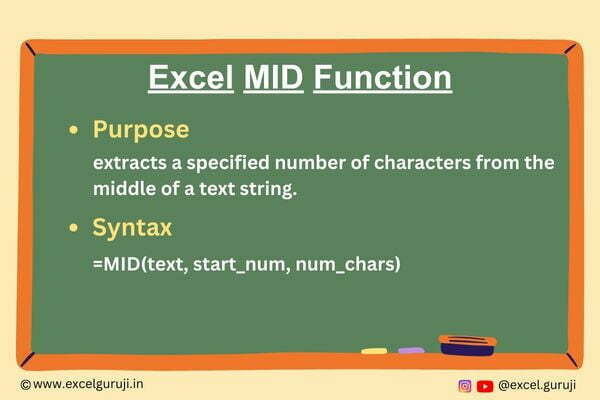
The MID function in Excel comes to the rescue when you need to extract a specific number of characters from the middle of a text string. This versatile function finds its application in various scenarios, from data manipulation to text refinement and even performing calculations that rely on extracting particular segments of text.

What Excel MID Function Returns

The Excel MID function is your go-to tool for retrieving a substring of characters from within a text string. Unlike the LEFT function, which starts from the beginning, and the RIGHT function, which operates from the end, the MID function lets you specify a starting point within the text and the length of the desired substring.

Syntax of Excel MID Function

The syntax of the Excel MID function is structured as follows

=MID(text, start_num, num_chars)

Input Arguments

Here are the input arguments for the Excel MID function:

👉 text: The text string can be a reference to a cell containing the text or a direct text entry enclosed in quotation marks. It can also be a formula that evaluates to a text string.

👉 start_num: This argument specifies the starting position within the text string from which you want to extract characters. It can be a positive integer value or a reference to a cell containing such a value.

👉 num_chars: The number of characters to be extracted from the text string, starting from the designated start_num. This argument must also be a positive integer or a reference to a cell containing one.

Examples of the MID Function in Excel

Here are a few illustrative examples showcasing the prowess of the MID function in Excel:

Example 1: Basic Usage

Assume that cell A1 contains the text “Excel Functions,” and you want to extract a portion of the text starting from the 7th character up to the next 5 characters. In another cell, use the formula

Example 2: Using a Cell Reference for Start and Length

Suppose you have a list of sentences in cell A1, and you want to extract a specific portion from a sentence based on the start position and length provided in cells B1 and C1, respectively. In cell D1, use the following formula:

Example 3: Extracting Domain from URLs

Imagine you have a list of URLs in column A, and you want to extract the domain name from each URL. You can use the FIND function to locate “http://” or “https://”, then apply the MID function. If A1 contains “https://www.example.com/page,” in cell B1, use the following formula:

Understanding of Formula

(1) MID(A1, FIND(“://”, A1) + 3, …)

• The MID function is used to extract a portion of the text from cell A1.
• FIND(“://”, A1) + 3 locates the position of the characters “://” in the URL and adds 3 to move the starting point beyond “://”.

(2) FIND(“/”, A1, FIND(“://”, A1) + 3)

• This nested FIND function is used to locate the position of the first forward-slash (“/”) that appears after “://”.
• FIND(“://”, A1) + 3 locates the position after “://” (i.e., the start of the domain).
• The second argument, A1, specifies the text in which to search for the forward slash.
• This part of the formula essentially identifies the end of the domain name.

(3) FIND(“/”, A1, FIND(“://”, A1) + 3) – FIND(“://”, A1) – 3

• This subtraction calculates the length of the domain name.
• FIND(“/”, A1, FIND(“://”, A1) + 3) identifies the position of the first forward slash after “://”, which marks the end of the domain
• FIND(“://”, A1) gives the position of “://” at the beginning of the URL.
• Subtracting these two positions, along with the 3 added earlier, gives the length of the domain.
  

Practice Workbook

Conclusion

In summary, the Excel MID function is an invaluable asset for extracting precise character sequences from within text strings. Whether you’re handling data, refining textual content, or conducting analyses, the MID function simplifies tasks and bolsters your mastery of Excel.

Just like any Excel function, proficiency comes through practice. Embrace experimentation and explore various applications of the MID function in your projects. Dive into using the MID function today and elevate your Excel skills to new heights!

Frequently Asked Questions (FAQs)

Q1: Can the MID function be used to extract characters from both sides of a text string?

A1: No, the MID function solely extracts characters from within the text string. For extracting from the right side, you should consider using the RIGHT function in Excel.

Q2: Is the MID function case-sensitive when working with letters?

A2: No, uppercase and lowercase letters are considered equivalent when extracting characters using the MID function.

Q3: What happens if the combined count of start_num and num_chars surpasses the text’s length?

A3: In such instances, the function will retrieve all characters from the designated start_num position until the end of the text.

Q4: Can I input cell references for the start_num and num_chars arguments?

A4: Certainly, both the start_num and num_chars arguments can be supplied with positive integer values stored in cells.

Q5: How can I extract characters from the end of a text string using Excel?

A5: To extract characters from the end, utilize the RIGHT function instead of the MID function.

Other Related Excel Functions

LEFT Function

RIGHT Function

UPPER Function

LEN Function

Join me on Instagram and YouTube for your daily dose of valuable tips and tricks! Catch insightful videos that will enhance your knowledge and skills. Don’t miss out – follow me now!

Excel RIGHT Function

When to Use the Excel RIGHT Function in Excel

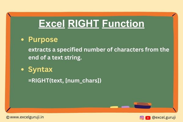
The RIGHT function in Excel is used when you need to extract a specific number of characters from the end of a text string. It can be used in various scenarios, such as manipulating data, cleaning up text, or performing calculations based on specific portions of a text.

What Excel RIGHT Function Returns

The Excel RIGHT function returns a substring of characters from the right side of a text string. The number of characters to extract is determined by the second argument, which is user-defined.

Syntax of Excel RIGHT Function

The syntax of the Excel RIGHT function is as follows

=RIGHT(text, [num_chars])

Input Arguments

Here are the input arguments for the Excel RIGHT function:

👉 text: The text string can be a reference to a cell containing the text or a direct text entry enclosed in quotation marks. It can also be a formula that evaluates to a text string.

👉 num_chars: The number of characters to extract must be a positive integer or a reference to a cell containing a positive integer.

Extra Notes

👉 If the specified num_chars is greater than the length of the text string, the function will return the entire text string.

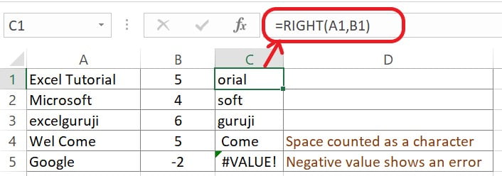
👉 Spaces are also counted as characters

👉 If the second argument is omitted, it is assumed to be 1

👉 If the value in the num_character argument is a non-numeric and negative number, the left function returns a #value! error

Examples of the RIGHT Function in Excel

Here are four examples of using the RIGHT function in Excel

Example 1: Basic Usage

Cell A1 contains the text “Excel Functions,” and you wish to retrieve the first 9 characters from the right. In the cell B1 utilize the following formula

Example 2: Using a Cell Reference for Length

Suppose you have a range of names in column A, and you aim to extract the rightmost characters based on the length specified in column B. Within column C, input the following formula:

Example 3: Dealing with Variable-Length Text:

Consider having a list of email addresses in column A, and your goal is to extract the domain name from each email. You can utilize the LEN function to used to determine the total length of the email address and the FIND function to locate the “@” symbol and then apply the RIGHT function. Given that A1 contains “example@email.com,” the formula in cell B2 would be

Excel RIGHT Function – Video Tutorial

Practice Workbook

Conclusion

In conclusion, the Excel RIGHT function is an indispensable tool for extracting specific character sequences from text strings. Whether you are managing data, working with names, or analyzing information, the RIGHT function can simplify your tasks and enhance your Excel proficiency.

Remember, mastering Excel functions takes practice, so do not hesitate to experiment and explore different applications of the RIGHT function in your own projects. Start utilizing the RIGHT function today and elevate your Excel skills to new heights!

Frequently Asked Questions (FAQs)

Q1: Can the RIGHT function be used to extract characters from the left side of a text?

A1: No, the RIGHT function is designed exclusively for extracting characters from the right side of the text.

Q2: Does the RIGHT function differentiate between uppercase and lowercase letters?

A2: No, the RIGHT function treats uppercase and lowercase letters as identical, operating in a case-insensitive manner.

Q3: What occurs if the designated character count exceeds the text’s length?

A3: In such cases, the function will return the complete original text.

Q4: Can cell references serve as the num_chars argument?

A4: No, the num_chars argument necessitates a positive integer value.

Q5: How can characters from the start of a text be extracted using Excel?

A5: For extracting characters from the start of a text, the LEFT function should be utilized instead of the RIGHT function.

Other Related Excel Functions

UPPER Function

MID Function

LEN Function

LOWER Function

PROPER Function

TRIM Function

FIND Function

SUBSTITUTE Function

REPLACE Function

Join me on Instagram and YouTube for your daily dose of valuable tips and tricks! Catch insightful videos that will enhance your knowledge and skills. Don’t miss out – follow me now!

Excel LEFT Function

When to Use the Excel LEFT Function in Excel

The LEFT function in Excel is used when you need to extract a specific number of characters from the beginning of a text string. It can be used in various scenarios, such as manipulating data, cleaning up text, or performing calculations based on specific portions of a text.

What Excel LEFT Function Returns

The Excel LEFT function returns a substring of characters from the left side of a text string. The number of characters to extract is determined by the second argument, which is user-defined.

Syntax of Excel LEFT Function

The syntax of the Excel LEFT function is as follows

=LEFT(text, [num_chars])

Input Arguments

Here are the input arguments for the Excel LEFT function:

👉 text: The text string can be a reference to a cell containing the text or a direct text entry enclosed in quotation marks. It can also be a formula that evaluates to a text string.

👉 num_chars: The number of characters to extract must be a positive integer or a reference to a cell containing a positive integer.

Extra Notes

👉 If the specified num_chars is greater than the length of the text string, the function will return the entire text string.

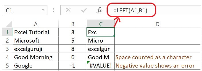
👉 Spaces are also counted as characters

👉 If the second argument is omitted, it is assumed to be 1

👉 If the value in the num_character argument is a non-numeric and negative number, the left function returns a #value! error

Examples of the LEFT Function in Excel

Here are four examples of using the LEFT function in Excel

Example 1: Basic Usage

Cell A1 contains the text “Excel Functions,” and you wish to retrieve the first 5 characters from the left. In the cell B1 utilize the following formula

Example 2: Using a Cell Reference for Length

Suppose you have a range of names in column A, and you aim to extract the leftmost characters based on the length specified in column B. Within column C, input the following formula:

Example 3: Dealing with Variable-Length Text:

Consider having a list of email addresses in column A, and your goal is to extract the username segment from each email. You can utilize the FIND function to locate the “@” symbol and then apply the LEFT function. Given that A1 contains “example@email.com” the formula in cell B2 would be

Excel LEFT Function – Video Tutorial

Practice Workbook

Conclusion

In conclusion, the Excel LEFT function is an indispensable tool for extracting specific character sequences from text strings. Whether you are managing data, working with names, or analyzing information, the LEFT function can simplify your tasks and enhance your Excel proficiency.

Remember, mastering Excel functions takes practice, so do not hesitate to experiment and explore different applications of the LEFT function in your own projects. Start utilizing the LEFT function today and elevate your Excel skills to new heights!

Frequently Asked Questions (FAQs)

Q1: Can the LEFT function be used to extract characters from the right side of a text?

A1: No, the LEFT function is designed exclusively for extracting characters from the left side of the text.

Q2: Does the LEFT function differentiate between uppercase and lowercase letters?

A2: No, the LEFT function treats uppercase and lowercase letters as identical, operating in a case-insensitive manner.

Q3: What occurs if the designated character count exceeds the text’s length?

A3: In such cases, the function will return the complete original text.

Q4: Can cell references serve as the num_chars argument?

A4: No, the num_chars argument necessitates a positive integer value.

Q5: How can characters from the end of a text be extracted using Excel?

A5: For extracting characters from the text’s end, the RIGHT function should be utilized instead of the LEFT function.

Other Related Excel Functions

UPPER Function

LOWER Function

MID Function

LEN Function

PROPER Function

TRIM Function

FIND Function

SUBSTITUTE Function

REPLACE Function

Join me on Instagram and YouTube for your daily dose of valuable tips and tricks! Catch insightful videos that will enhance your knowledge and skills. Don’t miss out – follow me now!