Greetings, Excel Enthusiast! Excel Online Test 3 awaits you with a mix of intermediate-level challenges. This quiz is designed to push your Excel capabilities further, covering topics like data manipulation and analysis and more.
Time's up
We highly value your feedback, so don’t hesitate to share your thoughts or questions. Your input guides us in creating quizzes that align with your learning objectives.
Thank you for choosing excelguruji.in as your learning hub. Enjoy Excel Online Test 3!
Unlock the next level of Excel mastery! Visit our quiz page by clicking below. With quizzes catering to all expertise levels, you are sure to find the perfect challenge.
The CHAR function proves valuable when you need to insert non-printable or special characters into your text strings, manipulate formatting, or create dynamic labels based on ASCII codes.
What Excel CHAR Function Returns
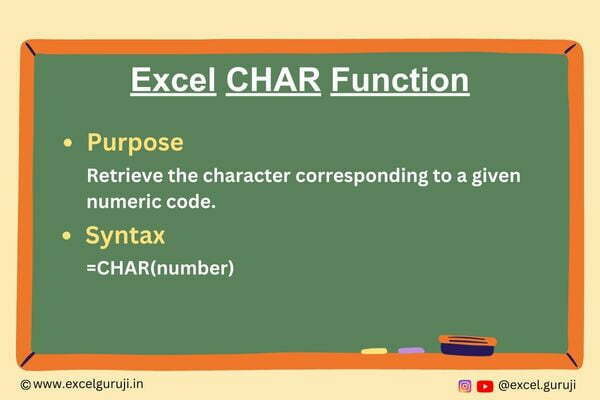
The Excel CHAR function returns a character based on the ASCII code provided as its argument. This code determines the character you want to extract or display.
Syntax of Excel CHAR Function
The syntax of the Excel CHAR function is as follows:
=CHAR(number)
Input Arguments
Here is the input argument for the Excel CHAR function:
👉 number: This is the ASCII code value representing the character you want to retrieve or display.
Extra Notes
👉 You can input a direct ASCII code value or use a cell reference containing the code.
👉 If the provided argument is not an integer within the range of 1 to 255, the Excel CHAR function displays a #VALUE! error.
👉 For numbers greater than 255, we can use the UNICHAR function.
👉 The function will give the result as a string/text value.
👉 Using incorrect or out-of-range codes may result in displaying unexpected characters.
Common Mistakes to Avoid
👉 Ensuring that the provided code corresponds to a valid character is crucial, as an incorrect code will yield an unintended result.
👉 Not formatting the cell appropriately to display the character may lead to the character not being visible.
Tips For Optimal Usage
To make the most out of the Excel CHAR function, consider the following tips:
👉 Utilize the CHAR function in combination with other Excel functions like CONCATENATE or SUBSTITUTE to create customized text strings.
👉 Use cell references for ASCII codes to easily modify characters in your spreadsheet without changing the formulas.
Examples of the Excel CHAR Function
Here are a few practical examples illustrating the Excel CHAR function is versatility:
Example 1: Displaying Special Characters
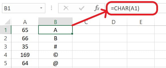
Let’s observe the outcomes obtained when applying the CHAR function to the following data:
Example 2: Insert a line break
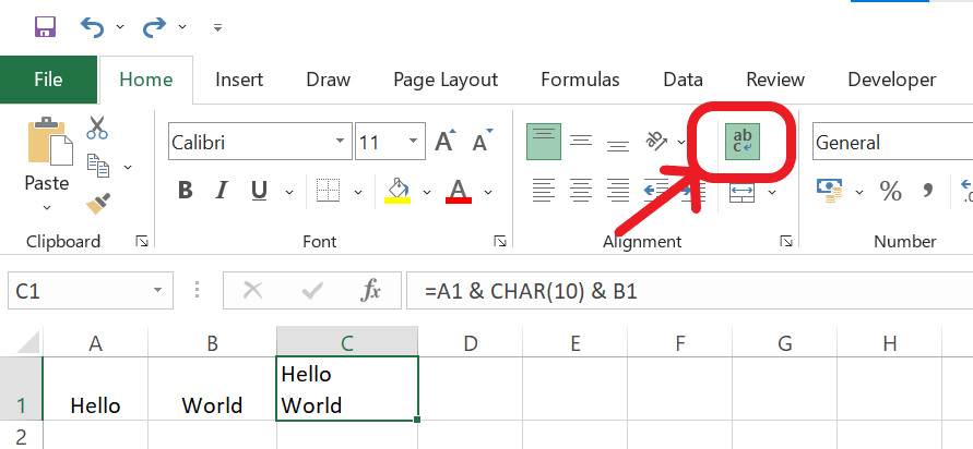
Suppose you have two pieces of text and you want to display them on separate lines within a single cell:
Here, the CHAR(10) function generates a line break character, which separates the text from cells A1 and A2 onto separate lines within cell B1.
In order to display line breaks within a single cell in Excel, you can make use of the “Wrap Text” option.
Once you enable the “Wrap Text” option, the cell’s contents will be displayed on multiple lines according to the line breaks you have added within the cell.
Conclusion
In summary, the Excel CHAR function empowers you to manipulate text and formatting by leveraging ASCII codes. By incorporating this function into your spreadsheet workflows, you can enhance the visual appeal and functionality of your data.
Remember, practice and experimentation will help you unlock the full potential of the CHAR function in Excel. Start utilizing the CHAR function today and add a new layer of versatility to your Excel skills.
Frequently Asked Questions (FAQs)
Q1: Can the CHAR function be used to retrieve characters based on Unicode codes?
A1: No, the CHAR function specifically works with ASCII codes and doesn’t support Unicode codes.
Q2: Can I use the CHAR function to input emojis or symbols?
A2: Yes, as long as you have the correct ASCII code for the emoji or symbol, you can use the CHAR function to display it.
Q3: Are there limitations to the ASCII codes that can be used with the CHAR function?
A3: Yes, the valid ASCII codes range from 1 to 255. Using codes outside this range won’t yield the desired characters.
Q4: Can I use formulas within the CHAR function to calculate ASCII codes dynamically?
A4: Yes, you can use formulas to calculate ASCII codes and input them into the CHAR function.
Q5: Can the CHAR function be combined with other text functions?
A5: Absolutely, the CHAR function can be combined with various text functions to create dynamic and customized text strings. Experimentation will unveil numerous possibilities.
Join me on Instagram and YouTube for your daily dose of valuable tips and tricks! Catch insightful videos that will enhance your knowledge and skills. Don’t miss out – follow me now!
You should turn to the CONCAT function whenever you need to join different text strings together. This function proves particularly handy when dealing with data that’s spread across different cells and needs to be consolidated into a coherent format.
What Excel CONCAT Function Returns
The Excel CONCAT function returns a single text string that results from the combination of two or more text strings. This combined string maintains the original formatting of the individual text components.
Syntax of Excel CONCAT Function
The syntax of the Excel CONCAT function is as follows:
=CONCAT(text1, [text2], …)
Input Arguments
Here are the input arguments for the Excel CONCAT function:
👉 text1, text2, …: These are the text strings or cell references that you want to combine.
Extra Notes
👉 You can include up to 255 text arguments.
👉 If any of the specified text arguments are empty cells, the CONCAT function will ignore them and only concatenate the non-empty text.
👉 There are no spaces or separators automatically added between the concatenated text strings. If you want to include spaces or other characters between the combined strings, you need to include them as separate text arguments.
Common Mistakes to Avoid
👉 Forgetting to Separate Text Arguments: Each text argument should be separated by a comma within the CONCAT function. Forgetting to do so will result in an error.
👉 Including Unnecessary Quotation Marks: Unlike some other Excel functions, you don’t need to enclose your text arguments in quotation marks. Using quotation marks would treat the text as a literal string and result in unexpected outputs.
👉 Neglecting Empty Cells: If you have empty cells among your text arguments, remember that CONCAT will not automatically add spaces or separators between non-empty text. Make sure to account for this in your formula.
Tips For Optimal Usage
To make the most out of the Excel CONCAT function, consider the following tips:
👉 Use CONCAT with Dynamic Data: If you have changing data that needs to be combined regularly, consider using cell references as your text arguments. This way, your concatenated results will update automatically.
👉 Utilize Spaces and Separators: If you want to include spaces, commas, or any other characters between your concatenated text strings, add them as separate text arguments within the CONCAT function.
👉 Combine with Other Functions: Combine CONCAT with other functions like TEXT, IF, or SEARCH to create complex concatenation scenarios. For instance, you can use CONCAT with IF to conditionally combine text strings.
Examples of the Excel CONCAT Function
Here are a few examples showcasing the versatility of the CONCAT function in Excel:
Example 1: Basic Usage
Suppose you have the first name “Mark” in cell A1 and the last name “Zuckerberg” in cell B1. You can use the CONCAT function to combine these names in cell C1 like this:
Example 2: Conditional Concatenation
Imagine you have a list of names, but not all entries have a middle name. You can use CONCAT along with IF to handle this situation:
Now let’s break down the formula step by step:
(1) IF(C1<>””, …)
This part of the formula checks if cell C1 (the middle name) is not empty. If it is not empty, the formula executes the first part after the comma.
(2) CONCAT(A1, ” “, C1, ” “, B1)
If there is a middle name, this concatenates the first name (cell A1), a space, the middle name (cell C1), another space, and the last name (cell B1).
(3) CONCAT(A1, ” “, B1)
If there is no middle name, this concatenates the first name (cell A1), a space, and the last name (cell B1).
Conclusion
In summary, the Excel CONCAT function streamlines the process of combining text strings, making your data manipulation tasks more efficient. By using CONCAT, you can save time and ensure the accuracy of your merged data. Remember, practice makes perfect, so experiment with CONCAT in different scenarios to enhance your Excel skills further. Start utilizing the CONCAT function today and take your Excel proficiency to the next level!
Remember that while mastering Excel functions takes practice, the CONCAT function can significantly enhance your data manipulation capabilities. Experiment and explore its various applications to become an Excel pro!
Frequently Asked Questions (FAQs)
Q1: Can the CONCAT function handle numbers and dates?
A1: Yes, the CONCAT function can combine text, numbers, dates, and any other type of data that Excel supports.
Q2: Can I combine more than two text strings using CONCAT?
A2: Absolutely! CONCAT allows you to combine multiple text strings. Just separate each text argument with a comma.
Q3: Does CONCAT add spaces between text strings automatically?
A3: No, CONCAT doesn’t add spaces or any other characters automatically. You need to include them as separate text arguments if desired.
Q4: Can I use cell references as text arguments?
A4: Yes, you can use cell references, and it is often recommended, especially if your data changes frequently.
Q5: Are there any limitations to the number of text arguments I can use with CONCAT?
A5: You can use up to 255 text arguments with the CONCAT function.
Join me on Instagram and YouTube for your daily dose of valuable tips and tricks! Catch insightful videos that will enhance your knowledge and skills. Don’t miss out – follow me now!
The Excel REPLACE function shines when you need to substitute a specific segment of text with another segment. This can be particularly useful in scenarios such as data cleaning, fixing formatting issues, or updating information within a text string.
What Excel REPLACE Function Returns
The Excel REPLACE function effectively replaces a portion of a text string with a new specified text. It does so by specifying the starting position of the replacement and the number of characters to replace.
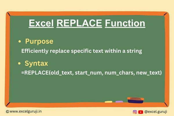
Syntax of Excel REPLACE Function
The syntax of the Excel REPLACE function is as follows:
Here’s a breakdown of the input arguments for the Excel REPLACE function:
👉 old_text: This is the original text string that you want to modify.
👉 start_num: This argument indicates the position within the old_text where the replacement should begin.
👉 num_chars: The number of characters to replace, starting from the start_num position.
👉 new_text: The new text that will replace the specified segment in the old_text.
Extra Notes
👉 If start_num is less than 1, or if it exceeds the length of the old_text, the function returns the original text without any changes.
👉 The num_chars argument can be set to 0, which will result in the insertion of the new_text at the start_num position.
👉 The start_num argument cannot be negative. If it is negative or zero, the function returns an error.
Common Mistakes to Avoid
👉 Misaligning start_num and num_chars: Ensure that the start_num and num_chars values are correctly specified to avoid unintended replacements.
👉 Omitting new_text: Forgetting to provide the new_text argument will result in an error or incomplete modification.
👉 Incorrectly calculating positions: Carefully calculate the positions within the text string to avoid replacing the wrong segment.
Tips For Optimal Usage
To make the most of the Excel REPLACE function, consider these tips:
👉 Combine with Other Functions: Integrate the REPLACE function with other Excel functions to create sophisticated transformations.
👉 Use Cell References: Utilize cell references for start_num, num_chars, and new_text to create dynamic replacements.
👉Preview Changes: Before implementing mass replacements, test the function on a smaller scale to ensure the results meet your expectations.
Examples of the Excel REPLACE Function
Let’s delve into some practical examples to illustrate the Excel REPLACE function’s versatility:
Example 1: Basic Replacement
Suppose you have a text string in cell A1: “Hello Excel Users.” You want to replace “Hello” with “Hi” using the REPLACE function. In cell B1, use the formula:
Example 2: Dynamic Replacement
Imagine you have a dataset of product codes in column A, and you want to update them by replacing the second character with “X.” In cell B2, which corresponds to the new code column, use the formula:
Example 3: Derive the Username from the Email Address
Let’s assume you have a list of email addresses in Column A, and you want to extract the user names (everything before the “@” symbol) in Column B. Here’s how you can achieve this:
Here’s what this formula does:
(1) FIND(“@”, A2)
This finds the position of the “@” symbol in the email address in cell A2.
(2) LEN(A2)
This calculates the length of the email address in cell A2.
(3) REPLACE(A2, FIND(“@”, A2), LEN(A2), “”)
This uses the REPLACE function to replace a portion of the email address starting from the “@” symbol’s position to the end with an empty string, effectively removing the domain part.
Difference Between Excel REPLACE Function & Excel SUBSTITUTE Function
In Excel, both the REPLACE and SUBSTITUTE functions are valuable tools for text manipulation, but they serve distinct purposes and operate differently. Understanding their differences is essential for effectively applying them in various scenarios.
Key Distinctions:
Segment vs. Substring: REPLACE operates by replacing a specific segment of characters based on position and length, while SUBSTITUTE replaces all instances of a given substring.
Position vs. Instances: REPLACE focuses on defined positions and lengths for replacements, while SUBSTITUTE centers on the substring itself and its occurrences.
Controlled vs. Global: REPLACE offers controlled modifications, swapping a particular segment while retaining the rest. SUBSTITUTE facilitates comprehensive replacements, rectifying errors or updating recurring content.
Use Cases: REPLACE excels in precise modifications where selective segments need replacement. SUBSTITUTE is advantageous for broad replacements, correcting consistent errors, or updating repetitive content.
In summary, the choice between the Excel REPLACE function and the SUBSTITUTE function hinges on whether you require specific segment modifications or global replacements of substrings within text strings.
Conclusion
In conclusion, the Excel REPLACE function is an indispensable asset for manipulating text strings precisely to meet your needs. From correcting errors to transforming data, this function empowers you to handle complex text modifications efficiently. As you familiarize yourself with the REPLACE function, you will be equipped to tackle a wide range of text-related challenges, enhancing your proficiency in Excel.
Remember, practice is key to mastering Excel functions. Don’t hesitate to experiment with the REPLACE function in various contexts to expand your skill set. Start leveraging the REPLACE function today and elevate your Excel capabilities to new heights!
Frequently Asked Questions (FAQs)
Q1: Can the REPLACE function be used to perform case-sensitive replacements?
A1: No, the REPLACE function in Excel is case-insensitive, meaning it treats uppercase and lowercase letters as identical.
Q2: Is it possible to replace characters from the right side of a text using the REPLACE function?
A2: While the REPLACE function is primarily designed for left-to-right replacements, you can achieve similar effects by using a combination of functions like RIGHT and LEFT.
Q3: What happens if the specified replacement length exceeds the remaining characters in the text?
A3: In such cases, the REPLACE function will replace the characters up to the end of the text and insert the new text accordingly.
Q4: Can the REPLACE function be used on non-text data, such as numbers or dates?
A4: Yes, the REPLACE function can be applied to any type of data that Excel recognizes, not just text.
Q5: Are there any limitations to the length of the new_text argument?
A5: The length of the new_text argument is not explicitly limited by the function. However, Excel’s overall cell character limit should be considered if you’re working with extensive replacements.
Join me on Instagram and YouTube for your daily dose of valuable tips and tricks! Catch insightful videos that will enhance your knowledge and skills. Don’t miss out – follow me now!
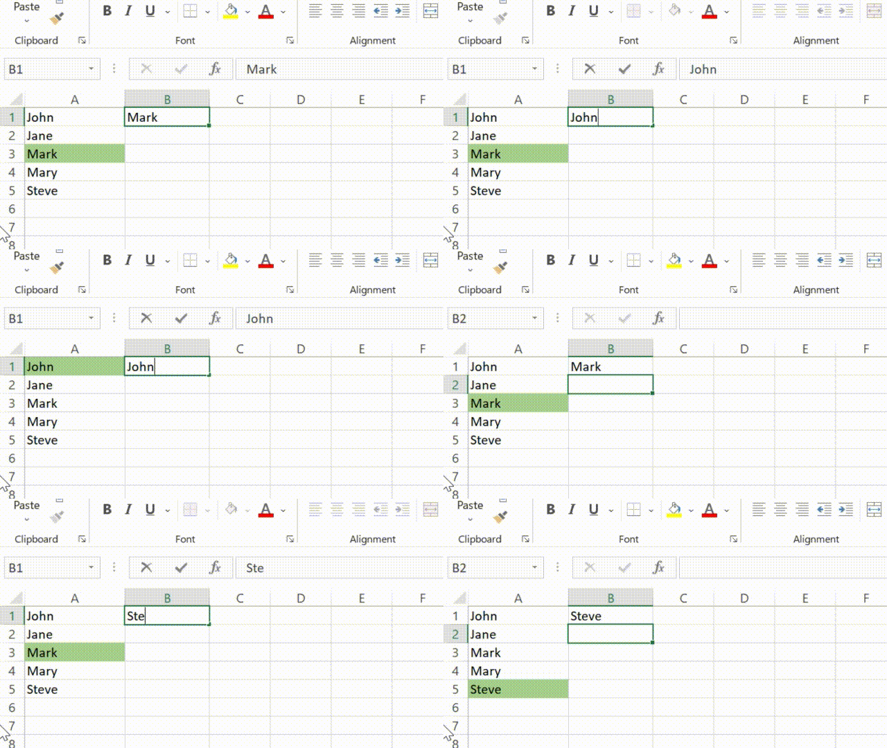
The Excel SEARCH function comes in handy when you need to determine the starting position of a specific substring within a text string. This can be immensely useful for tasks such as data extraction, conditional formatting, and more. By providing the position of the sought substring, the Excel SEARCH function enables you to precisely manipulate your data.
What Excel SEARCH Function Returns
In essence, the Excel SEARCH function returns the position of the first character of the searched substring within the given text. If the substring is not found, the function returns an error value, making it an excellent tool for validation and error checking in your worksheets.
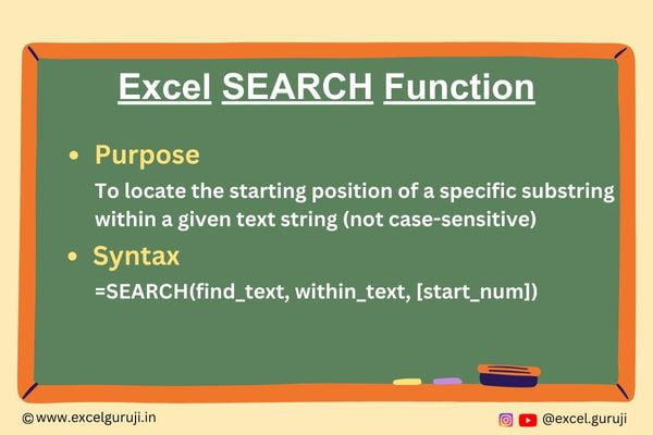
Syntax of Excel SEARCH Function
The syntax of the Excel SEARCH function is as follows:
=SEARCH(find_text, within_text, [start_num])
Input Arguments
Let’s break down the input arguments for the Excel SEARCH function:
👉 find_text: This is the substring you want to find within the within_text. It can be a direct text entry, a cell reference, or a formula that evaluates to text.
👉 within_text: This is the text string in which you want to search for the find_text.
👉 start_num (optional): This argument lets you specify the starting position for the search within the within_text. If omitted, the search starts from the beginning. It’s especially useful when you want to find multiple occurrences of a substring.
Extra Notes
👉 If the find_text is not found within the within_text, the SEARCH function returns the #VALUE! error.
👉 The SEARCH function is case-insensitive, meaning it treats uppercase and lowercase letters as equivalent.
👉 The start_num argument cannot be negative. If it is negative or zero, the function returns an error.
Examples of the Excel SEARCH Function
Let’s explore a few examples of using the SEARCH function in Excel:
Example 1: Basic Usage
Suppose cell A1 contains the text “Excel functions are powerful.” You want to find the position of the word “functions.” In cell B1, use the formula:
Example 2: Using the start_num Argument
Let’s say you want to find the second occurrence of “functions” in cell A1. In cell B1, use the formula:
Here’s what each part of the formula does:
(1) SEARCH(“functions”, A1)
This inner SEARCH function searches for the first occurrence of the word “functions” within the text in cell A1. Let’s say this position is 7 (counting spaces and characters).
(2) SEARCH(“functions”, A1) + 1
This part adds 1 to the position found in step 1. In our example, it would be 8. This adjustment is made so that the search for the second occurrence starts from the character immediately after the first occurrence.
This outer SEARCH function starts searching for the word “functions” again, but this time, it starts from the position calculated in step 2 (8). This effectively skips the first occurrence and looks for the second occurrence.
Example 3: Extracting Text Between Brackets
Suppose you have a list of product codes in column A, and the product codes are enclosed in square brackets. Your goal is to extract the product codes from within the brackets.
Let’s break down the formula step by step:
(1) SEARCH(“[“, A1)
This part of the formula searches for the position of the opening square bracket [ within the text in cell A1.
(2) SEARCH(“]”, A1):
This part of the formula searches for the position of the closing square bracket ] within the text in cell A1.
(3) SEARCH(“]”, A1) – SEARCH(“[“, A1) – 1
This calculates the length of the text between the opening and closing square brackets. It subtracts the position of the opening square bracket from the position of the closing square bracket and then subtracts 1 to exclude the brackets themselves.
This part of the formula uses the MID function to extract the text between the brackets. The MID function takes three arguments: the text from which to extract (A1), the starting position (found in step 1), and the number of characters to extract (calculated in step 3).
Excel Search Function – Video Tutorial
Difference Between SEARCH Function & FIND Function
Both the SEARCH and FIND functions in Excel are used to locate the position of a specific substring within a text string. However, there is a crucial difference between the two functions: case-sensitivity.
Use SEARCH when you want a case-insensitive search. For instance, if you’re searching for the word “mango”, SEARCH will find “mango”, “Mango” and “MANGO”.
Use FIND when you want a case-sensitive search. For example, if you’re looking for the word “mango”, FIND will only find “mango” and not “Mango” or “MANGO”.
Conclusion
In conclusion, the Excel SEARCH function is an invaluable tool for locating substrings within text strings. Whether you are cleaning up data, validating entries, or performing advanced analysis, the SEARCH function empowers you with precise control over your text data.
Remember, the true mastery of Excel functions comes from hands-on practice. So, don’t hesitate to experiment and apply the SEARCH function in various scenarios. Start using the SEARCH function today to unlock new dimensions of efficiency and accuracy in your Excel projects!
Frequently Asked Questions (FAQs)
Q1: Can the SEARCH function be used for case-sensitive searches?
A1: No, the SEARCH function is case-insensitive and treats uppercase and lowercase letters as the same.
Q2: What does the SEARCH function return if the find_text is not found?
A2: If the find_text is not found, the SEARCH function returns the #VALUE! error.
Q3: Can the start_num be a negative value?
A3: No, the start_num must be a positive integer. Negative values will result in an error.
Q4: Can the SEARCH function be used for finding multiple occurrences of a substring?
A4: Yes, by adjusting the start_num argument, you can find multiple occurrences of a substring within the within_text.
Q5: Is there a way to perform case-sensitive searches in Excel?
A5: Yes, for case-sensitive searches, you can use the FIND function instead of SEARCH.
Join me on Instagram and YouTube for your daily dose of valuable tips and tricks! Catch insightful videos that will enhance your knowledge and skills. Don’t miss out – follow me now!
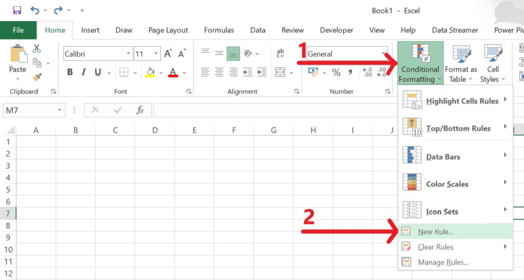
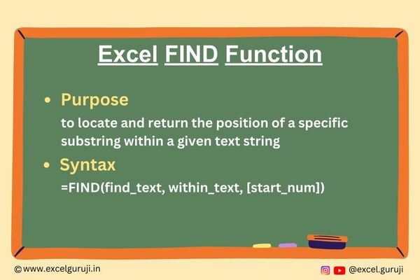
The FIND function comes to the rescue when you need to determine the position of a specific character or substring within a text string. Whether you are extracting information, replacing characters, or performing complex data transformations, FIND offers a powerful way to navigate through your data.
What Excel FIND Function Returns
Unlike some functions that return values, the FIND function returns the position of the first occurrence of a specified substring within a text string. This position is counted from the first character of the text string, with spaces included in the count.
Syntax of Excel FIND Function
The syntax of the Excel FIND function is as follows:
=FIND(find_text, within_text, [start_num])
Input Arguments
Here are the input arguments for the Excel FIND function:
👉 find_text: The substring you’re searching for within the within_text. This can be a direct entry enclosed in quotation marks, a cell reference, or a formula resulting in a text string.
👉 within_text: The text string that you want to search within. Similar to find_text, this can be a direct entry, a cell reference, or a formula.
👉 start_num (optional): The character position within within_text where the search should begin. If omitted, the search starts from the first character.
Extra Notes
👉 If find_text is not found within within_text, the function returns an error (#VALUE!).
👉 If start_num exceeds the length of within_text, the function also returns an error (#VALUE!).
Examples of the Excel FIND Function
Let’s explore some examples showcasing the utility of the Excel FIND function:
Example 1: Basic Usage
Suppose cell A1 contains the text “Excel Functions,” and you want to find the position of the word “Functions.” Utilize the formula:
Example 2: Extracting Substring Using FIND
Suppose you have URLs in column A, and you want to extract the domain from each URL. You can use FIND in combination with LEFT and MID functions:
Here’s the breakdown of the formula:
(1) FIND(“://”, A1)
This part of the formula locates the position of the string “://” within the URL.
In the given URL “https://www.example.com/page”, the result of this portion is 6.
Adding 3 to this result (+3) ensures that we start searching after “://” and the following 3 characters.
(2) FIND(“/”, A1, FIND(“://”, A1)+3)
This part locates the position of the first “/” character after the protocol and subdomain.
Using the result of the previous portion (position after “://”), which is 9, as the starting position.
In the given URL, the result of this portion is 21, as it’s the position of the first “/” after “://”.
This part combines the MID function with the calculated positions and length to extract the domain.
MID(A1, FIND(“://”, A1)+3, FIND(“/”, A1, FIND(“://”, A1)+3) – FIND(“://”, A1) – 3) extracts a substring from the URL.
The starting position is the result of the first portion (9) and the length is the result of the third portion (12).
So, it extracts the substring starting at position 9 and of length 12.
Difference Between FIND Function & SEARCH Function
Both the FIND and SEARCH functions in Excel are used to locate the position of a specific substring within a text string. However, there is a crucial difference between the two functions: case-sensitivity.
Use FIND when you want a case-sensitive search. For example, if you’re looking for the word “apple”, FIND will only find “apple” and not “Apple” or “APPLE”.
Use SEARCH when you want a case-insensitive search. For instance, if you’re searching for the word “apple”, SEARCH will find “apple”, “Apple” and “APPLE”.
The Excel FIND function empowers you to navigate and manipulate text strings with precision. Its ability to locate specific characters within a text string is invaluable for data processing, text analysis, and more. As with any Excel function, practice is key to mastery. Experiment, explore, and elevate your Excel skills by incorporating the Excel FIND function into your toolkit.
Remember, embracing Excel functions like FIND takes practice and experimentation. As you become familiar with its nuances, you will unlock new possibilities for data manipulation and analysis. Start using the FIND function today and propel your Excel proficiency to greater heights!
Frequently Asked Questions (FAQs)
Q1: Can the FIND function locate the position of the last occurrence of a substring?
A1: No, the FIND function identifies the position of the first occurrence only. For the position of the last occurrence, consider using the combination of FIND and RIGHT functions.
Q2: Is the FIND function case-sensitive?
A2: Yes, by default, the FIND function is case-sensitive. To perform a case-insensitive search, consider using the SEARCH function.
Q3: What happens if the searched substring is not found?
A3: In such cases, the FIND function returns an error (#VALUE!).
Q4: Can variables be used as arguments in the FIND function?
A4: Yes, you can use variables, cell references, or direct entries as arguments.
Q5: Can FIND be employed to search for multiple substrings at once?
A5: No, FIND searches for a single substring at a time. To search for multiple substrings, consider nesting FIND within other functions.
Q6: Does FIND support wildcard characters for searching?
A6: No, FIND doesn’t support wildcard characters. For wildcard searches, explore the capabilities of other Excel text functions.
Join me on Instagram and YouTube for your daily dose of valuable tips and tricks! Catch insightful videos that will enhance your knowledge and skills. Don’t miss out – follow me now!
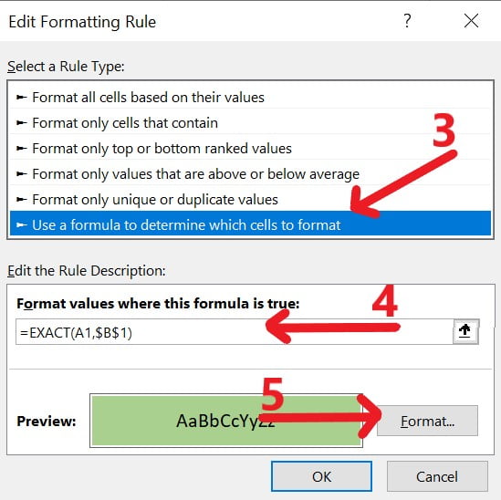
When to Use the Excel SUBSTITUTE Function in Excel
The SUBSTITUTE function in Excel is your go-to tool when you need to replace specific instances of text within a larger text string. This function proves invaluable in scenarios where you want to make selective changes, remove unwanted characters, or update outdated information.
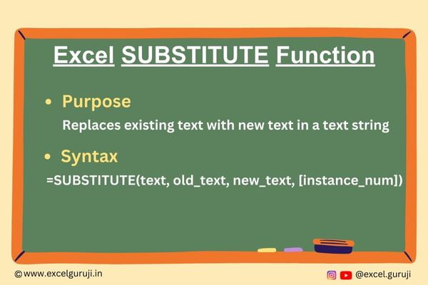
What Excel SUBSTITUTE Function Returns
The Excel SUBSTITUTE function replaces occurrences of a specified old text with new text in a given text string. You have the freedom to decide how many instances you want to replace. This makes it perfect for tasks such as standardizing data or correcting consistent typos.
Syntax of Excel SUBSTITUTE Function
The syntax of the Excel SUBSTITUTE function is as follows:
Here are the input arguments for the Excel SUBSTITUTE function:
👉 text: The text string that contains the instances you want to replace. This can be a direct text entry, a cell reference containing text, or a formula resulting in text.
👉 old_text: The specific text you want to replace within the text argument.
👉 new_text: The text you want to substitute in place of old_text.
👉 instance_num (optional): This parameter allows you to specify which occurrence of old_text you want to replace. If omitted, all instances of old_text will be replaced.
Extra Notes
👉 If old_text is not found within the text string, no changes will occur.
👉 If you provide an instance_num that is greater than the number of occurrences of old_text, no replacement will occur.
👉 The SUBSTITUTE function is case-sensitive. “Apple” and “apple” are treated as distinct text.
Common Mistakes to Avoid
👉 Misplacing quotation marks: Ensure that you properly enclose your text entries, old and new, in double quotation marks.
👉 Omitting the new_text argument: Every instance of old_text needs a corresponding replacement defined in new_text.
👉 Incorrect instance_num: If you want to replace a specific occurrence, make sure to count correctly and provide the appropriate instance number.
Tips For Optimal Usage
To make the most of the SUBSTITUTE function, consider these tips:
👉 Combine SUBSTITUTE with other functions like FIND or LEN for more intricate text manipulations.
👉 Experiment with relative and absolute cell references to automate replacements across multiple cells.
👉 Always double-check your new_text to avoid inadvertently changing data.
Examples of the Excel SUBSTITUTE Function
Let’s walk through a few examples to demonstrate the prowess of the Excel SUBSTITUTE function.
Example 1: Basic Usage
Suppose you have a list of product names containing “pro” that you want to change to “professional”. In cell B1, input:
Remember, The “Find and Replace” option is great for quick and simple text replacements, if you need to perform more intricate replacements or apply conditional transformations, using functions like SUBSTITUTE allows you to craft more dynamic and versatile solutions.
Example 2: Removing Unwanted Characters
In a list of product codes, there are unnecessary underscores. You want to remove all underscores from the codes.
Example 3: Replacing Multiple Special Characters
Suppose you have a text string that contains special characters like !, @, #,$ and you want to replace all of them with a space.
Here’s the breakdown of the formula:
(1) SUBSTITUTE(A1, “!”, ” “)
This innermost SUBSTITUTE function replaces all occurrences of the exclamation mark “!” in cell A1 with a space ” “. The result is a text string with exclamation marks replaced by spaces.
(2) SUBSTITUTE(result_1, “@”, ” “)
The result from the previous step (result_1) is then further processed by the next SUBSTITUTE function. It replaces all occurrences of the at symbol “@” with a space ” “. This continues the process of replacing characters with spaces.
(3) SUBSTITUTE(result_2, “#”, ” “)
The result from the previous step (result_2) is further processed to replace all occurrences of the hash symbol “#” with a space ” “.
(4) SUBSTITUTE(result_3, “$”, ” “)
The result from the previous step (result_3) is once again processed to replace all occurrences of the dollar sign “$” with a space ” “.
(5) TRIM(result_4)
Finally, the TRIM function is applied to the result from the last SUBSTITUTE operation (result_4). The TRIM function removes any leading or trailing spaces and ensures that there is only a single space between words.
The SUBSTITUTE function doesn’t support replacing multiple characters simultaneously using an array constant [like =SUBSTITUTE(A1, {“!”,”@”,”#”,”$”}, ” “)]
If you want to replace multiple special characters with a single SUBSTITUTE function, you would need to nest SUBSTITUTE functions as shown in the earlier examples.
Example 4: Replacing Specific Occurrences
You have a text string “A A A A A” and want to replace the fourth occurrence of “A” with “a”. In cell B1, input:
Conclusion
The Excel SUBSTITUTE function empowers you to manipulate text efficiently, giving you the ability to make precise replacements within text strings. By mastering this function, you open the door to a world of data cleaning, transformation, and consistency. With practice and creativity, you will uncover its potential to elevate your Excel skills to new heights.
Feel free to experiment, refine, and integrate SUBSTITUTE into your own projects. Excel is a toolbox, and SUBSTITUTE is a powerful tool that can help you achieve remarkable text transformations with ease.
Frequently Asked Questions (FAQs)
Q1: Can SUBSTITUTE handle case-insensitive replacements?
A1: No, SUBSTITUTE is case-sensitive. “Apple” and “apple” are treated differently.
Q2: What if old_text appears multiple times within text but I want to replace only the third occurrence?
A2: You can achieve this by specifying instance_num as 3 in your SUBSTITUTE formula.
Q3: Can I use cell references for old_text and new_text?
A3: Yes, you can use cell references as long as they contain the appropriate text values.
Q4: Does SUBSTITUTE work with numbers as well?
A4: Yes, SUBSTITUTE can replace numbers just like text, as long as you treat them as text entries.
Join me on Instagram and YouTube for your daily dose of valuable tips and tricks! Catch insightful videos that will enhance your knowledge and skills. Don’t miss out – follow me now!
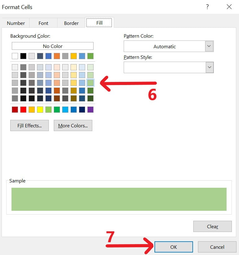
The TRIM function comes to the rescue when you are dealing with text strings that have unnecessary leading or trailing spaces. These spaces can throw a wrench in your data analysis, causing issues when trying to match or compare values.
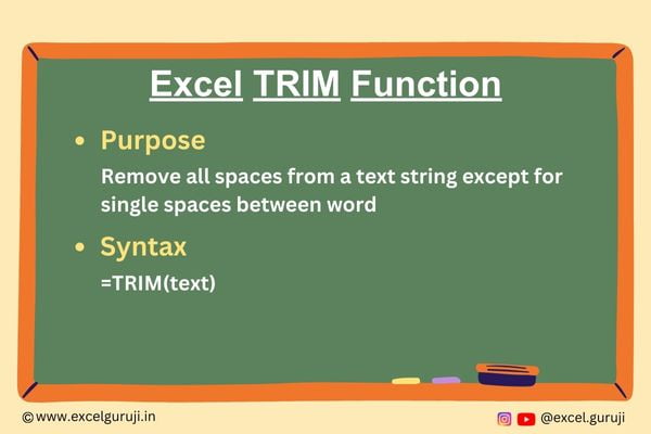
What Excel TRIM Function Returns
In essence, the Excel TRIM function does just one thing – it removes any extra spaces from a text string, leaving only a single space between words and no leading or trailing spaces.
Syntax of Excel TRIM Function
The syntax of the Excel TRIM function is quite straightforward:
=TRIM(text)
Input Arguments
Here are the input arguments for the Excel TRIM function:
👉 text: This is the text string that you want to trim. It can be a direct text entry, a cell reference containing text, or a formula that evaluates to a text string.
Extra Notes
👉 The TRIM function doesn’t affect spaces between words, ensuring your text remains coherent.
👉 If your text contains non-breaking spaces (CHAR(160)), TRIM won’t remove those. You might need to use SUBSTITUTE or another approach to deal with them.
Common Mistakes to Avoid
👉Misapplying TRIM: Remember, TRIM only removes leading and trailing spaces. If you have extra spaces between words that you want to reduce to a single space, you might need to combine TRIM with other functions.
👉 Overusing TRIM: While TRIM is a lifesaver for cleaning up data, don’t overdo it. Applying TRIM to cells that don’t have extra spaces can slow down your calculations unnecessarily.
👉 Neglecting Non-Breaking Spaces: Keep in mind that TRIM doesn’t remove non-breaking spaces (CHAR(160)) which might exist in your text.
Tips For Optimal Usage
For a smooth experience with the Excel TRIM function, keep these tips in mind:
👉 Combine with FIND or SEARCH: If you need to remove specific characters along with spaces, consider combining TRIM with the FIND or SEARCH functions to locate those characters.
👉 Use on Imported Data: When you import data from external sources, extra spaces can often sneak in. Apply TRIM after importing to ensure clean data.
👉 Utilize on Concatenated Data: If you’re concatenating text strings from different sources, spaces can creep in. TRIM will help maintain the integrity of your concatenated results.
Examples of the TRIM Function in Excel
Let’s look at a couple of examples to see how the TRIM function works:
Example 1: Basic Usage
Suppose cell A1 contains the text ” Excel TRIM Function ” with extra spaces. You can use the following formula in cell B1:
Example 2: Extracting Initials from Full Names
Suppose you have a list of full names in column A (e.g., “Samuel Johnson”) and you want to extract the initials from each name. You can use TRIM in combination with LEFT and MID functions
Here’s the breakdown of the formula:
(1) TRIM(A1)
The TRIM function is applied to the text in cell A1 to remove any leading or trailing spaces.
(2) LEFT(TRIM(A1), 1)
The LEFT function extracts the first character of the trimmed text (the first initial).
(3) “.”
A period is concatenated to the first initial using the ampersand (&) operator.
(4) MID(TRIM(A1), FIND(” “, TRIM(A1), 1) + 1, 1)
The MID function extracts a portion of the trimmed text. The FIND function is used to locate the position of the first space within the trimmed text. Adding 1 to this position gives the starting position of the second word (second initial). The MID function then extracts 1 character from this position.
Conclusion
The Excel TRIM function might not be the flashiest function, but it is a true workhorse when it comes to maintaining clean and consistent text data. By eradicating unwanted spaces, TRIM ensures that your analyses and calculations are accurate and error-free.
Remember, just like any Excel function, the more you use TRIM, the more comfortable you’ll become with it. Incorporate it into your data cleaning routine, and you’ll soon wonder how you ever managed without it. Happy trimming!
Frequently Asked Questions (FAQs)
Q1: Does the TRIM function affect spaces between words?
A1: No, the TRIM function only removes leading and trailing spaces. It ensures that there’s only one space between words in the text. Internal spaces within the text remain unchanged..
Q2: Can the TRIM function be used on numeric values?
A2: No, the TRIM function is designed specifically for text values. Applying it to numeric values or other non-text entries will have no effect.
Q3: Can I use TRIM in combination with other text functions?
A3: Absolutely! TRIM can be a powerful component of more complex text manipulation formulas. It’s often used in combination with other functions like SUBSTITUTE, CONCATENATE (or the “&” operator), FIND, and MID to achieve specific text cleaning or transformation tasks.
Q4: Does the TRIM function have any impact on formulas that reference the trimmed cell?
A4: Yes, using TRIM on a cell will modify the text within that cell. If you have formulas referencing the original cell, they will now reference the trimmed text. Keep this in mind if you have downstream formulas relying on the untrimmed text.
Q5: Can TRIM be applied to a range of cells?
A5: Yes, you can apply the TRIM function to a range of cells using array formulas. For example, if you have a range of text in cells A1:A10, you can enter the formula =TRIM(A1:A10) as an array formula by pressing Ctrl+Shift+Enter instead of just Enter.
Join me on Instagram and YouTube for your daily dose of valuable tips and tricks! Catch insightful videos that will enhance your knowledge and skills. Don’t miss out – follow me now!
Get ready for Excel Online Test 2! This quiz delves deeper into Excel functionalities, challenging your understanding of formulas and functions. Your commitment to honing your Excel skills is commendable.
Time's up
Feel free to express your experiences, insights, or ask for clarification on any question. Your engagement is essential for us to continually improve and deliver content that resonates with you.
Thanks for being an integral part of the excelguruji.in community. Best of luck with Excel Online Test 2!
Ready for a fresh challenge? Click below to explore our array of quizzes, each designed to amplify your Excel prowess. Whether you are a novice or an expert, there is a quiz waiting for you.
Welcome to Excel Online Test 1! This quiz is designed to kickstart your Excel journey, covering fundamental concepts and basic functions. We appreciate your eagerness to learn and hope this quiz adds value to your Excel skills.
Time's up
Take your time, answer with confidence, and feel free to share your thoughts or questions after completing the test. Your feedback is vital for us to tailor future quizzes to your needs.
Thank you for your dedication to excelguruji.in, and we hope you enjoy Excel Online Test 1!
Craving more Excel excitement? Dive into our extensive quiz collection by clicking below. Unleash your potential with quizzes tailored for every skill level.