Excel Guruji - Excel Guruji

Mastering the Excel NOT Function: A Comprehensive Guide for Efficient Data Analysis

October 5, 2023 by Excel Guruji

Excel NOT Function

When to Use the Excel NOT Function in Excel

Excel NOT function comes in handy when you need to reverse the logical value of a condition or expression. It is primarily used in conjunction with other logical functions and formulas to make decisions based on the opposite of a given condition.

Whether you are creating complex formulas or simply checking if a condition is false, the NOT function can streamline your Excel tasks.

What Excel NOT Function Returns

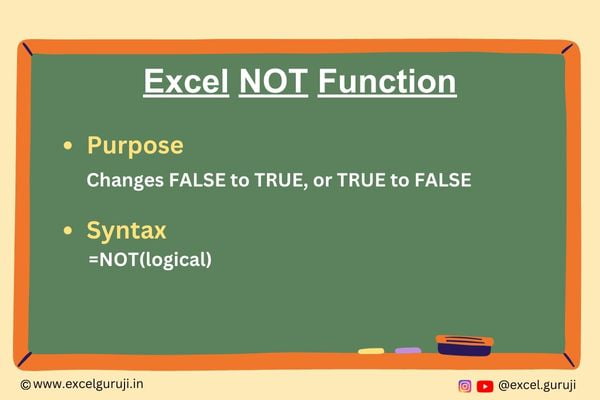
Excel NOT function returns the opposite of a logical value. If the input value is TRUE, it returns FALSE, and if the input value is FALSE, it returns TRUE. In other words, it negates the logical value provided as its argument.

Syntax of Excel NOT Function

The syntax of the Excel NOT function is straightforward:

=NOT(logical)

Input Arguments

Here is the input argument for the Excel NOT function:

● logical: This is the logical value or expression that you want to negate. It can be a cell reference containing a logical value, a formula that evaluates to a logical value, or a direct logical value (TRUE or FALSE).

Extra Notes

● When you have FALSE as the logical value, NOT will give you TRUE. And when you have TRUE as the logical value, NOT will give you FALSE.

Examples of the Excel NOT Function

Let’s explore a few examples to illustrate how to use the Excel NOT function effectively.

Example 1: Basic Usage

Below example showcases how NOT can reverse logical outcomes in Excel, enhancing decision-making.

Formula in Cell D2: =NOT(A2=”Apple”), This formula uses the NOT function to negate the result of the formula in cell B2. Since the result in cell B2 is TRUE, the NOT function turns it into FALSE.

Formula in Cell D3: =NOT(A3=”Apple”), This formula, like in the previous row, uses the NOT function to negate the result of the formula in cell B3. Since the result in cell B3 is FALSE, the NOT function turns it into TRUE.

Conclusion

In conclusion, the Excel NOT function is an essential tool for working with logical values and conditions in your Excel spreadsheets. It allows you to reverse the outcome of logical expressions, enabling you to make more informed decisions and streamline your data analysis tasks.

As with any Excel function, practice is key to mastering the NOT function. Experiment with different scenarios and integrate it into your formulas to see how it can enhance your Excel proficiency. Start using the NOT function today to take your Excel skills to the next level!

Frequently Asked Questions (FAQs)

Q1: Can the NOT function be used with text strings?

A1: No, the NOT function is designed for working with logical values (TRUE or FALSE) and cannot be directly applied to text strings.

Q2: What does the NOT function return if the input is not a valid logical value?

A2: If the input provided to the NOT function is not a valid logical value (neither TRUE nor FALSE), it will return a #VALUE! error.

Q3: Can the NOT function be used to negate multiple conditions at once?

A3: Yes, you can use the NOT function in combination with other logical functions like Excel AND Function and Excel OR Function to negate multiple conditions and create complex logical expressions.

Q4: Is the NOT function case-sensitive?

A4: No, the NOT function is case-insensitive and treats TRUE and FALSE as equivalent regardless of letter casing.

Join me on Instagram, YouTube and WhatApp Channel for your daily dose of valuable tips and tricks! Catch insightful videos that will enhance your knowledge and skills. Don’t miss out – follow me now!

Excel OR Function: Simplify Decision-Making with Multiple Conditions

October 5, 2023 by Excel Guruji

Excel OR Function

When to Use the Excel OR Function in Excel

Excel OR function comes in handy in various situations where you want to check if any of the specified conditions are met. Here are some common scenarios where you might use the OR function:

Conditional Formatting: You can use the OR function to apply conditional formatting to a cell or range of cells based on multiple conditions.

Data Filtering: When filtering data, you can use the OR function to filter rows that meet any of the specified criteria.

Logical Tests: In logical tests and formulae, the OR function helps simplify complex decision-making processes.

Error Handling: It can be used to handle errors by checking for multiple error conditions.

What Excel OR Function Returns

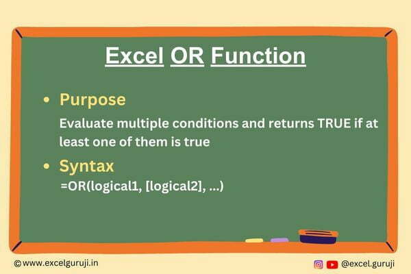
The Excel OR function returns a Boolean value: TRUE if at least one of the conditions evaluates to TRUE, and FALSE if none of the conditions are met.

Syntax of Excel OR Function

The syntax of the Excel OR function is straightforward:

=OR(logical1, [logical2], …)

Input Arguments

Here are the input arguments for the Excel OR function:

● logical1, logical2, …: These are the conditions you want to evaluate. You can specify up to 255 conditions separated by commas. Each condition can be a logical expression, a cell reference, or a value.

Extra Notes

● If any of the conditions are text values, numbers, or empty cells, the OR function considers them as either TRUE or FALSE based on whether they contain data.

● If all the conditions are empty cells, the OR function returns FALSE.

● To check if a specific value is found within an array, you can utilize an OR array formula. Inputting an array formula is accomplished by pressing CTRL+SHIFT+ENTER.

● Text values must be enclosed in quotation marks ” “

Examples of the Excel OR Function

Let’s dive into some examples to illustrate how the OR function works:

Example 1: Basic Usage

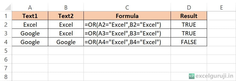
Suppose you want to check if either cell A1 or cell B1 contains the word “Excel.” You can use the following formula in cell C1:

This formula returns TRUE if any one condition is met.

Example 2: Use With IF Function

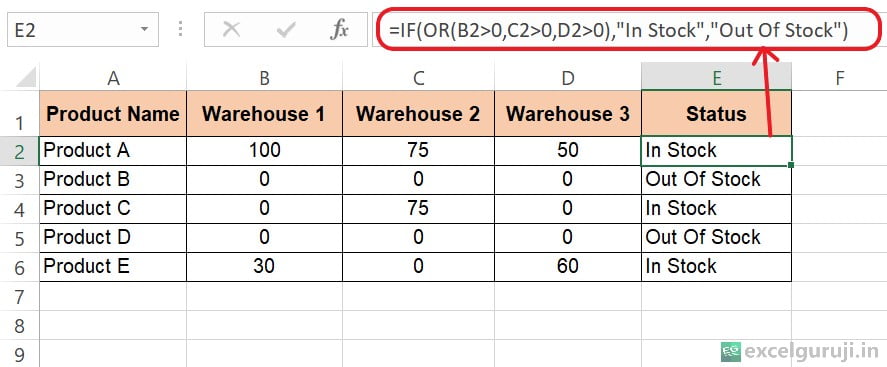
Below is the formula that determines the stock status of each product based on the available quantities in the warehouses.

Now, let’s break down the formula used in the “Status” column:

=IF(OR(B2>0,C2>0,D2>0),”In Stock”,”Out Of Stock”)

IF Function: This is an Excel function used for conditional statements. It checks a specified condition and returns one value if the condition is TRUE and another value if it is FALSE.

OR Function: This function checks if any of the conditions within it are TRUE. In this case, it checks if any of the quantities in Warehouse 1, Warehouse 2, or Warehouse 3 are greater than 0.

“In Stock”: If any of the conditions in the OR function are TRUE (i.e., if any of the warehouses have a quantity greater than 0), the formula returns “In Stock”.

“Out Of Stock”: If none of the conditions in the OR function are TRUE (i.e., all warehouses have a quantity of 0), the formula returns “Out Of Stock”.

Example 3: Conditional Formatting to Highlight Weekends

Click here for more detail

Conclusion

In conclusion, the Excel OR function is a versatile tool for making decisions based on multiple conditions. Whether you are applying formatting, filtering data, or creating complex formulas, the OR function simplifies your tasks and enhances your Excel proficiency.

As with any Excel function, practice is key to mastery. Experiment with different applications of the OR function in your own projects to unlock its full potential. Start using the OR function today and take your Excel skills to the next level!

Frequently Asked Questions (FAQs)

Q1: Can the OR function evaluate more than 255 conditions?

A1: No, the OR function can evaluate up to 255 conditions. If you need to evaluate more conditions, consider using nested OR functions.

Q2: Can the OR function be used with numeric values?

A2: Yes, the OR function can be used with numeric values.

Q3: Can the OR function be combined with other logical functions like AND?

A3: Yes, you can combine the OR function with other logical functions like AND to create more complex logical expressions.

Q4: What if I want to check if all conditions are met instead of just one?

A4: In that case, you should use the Excel AND function, which returns TRUE only if all conditions are met.

Mastering the Excel AND Function: A Comprehensive Guide for Effective Spreadsheet Logic

October 5, 2023October 4, 2023 by Excel Guruji

Excel AND Function

When to Use the Excel AND Function in Excel

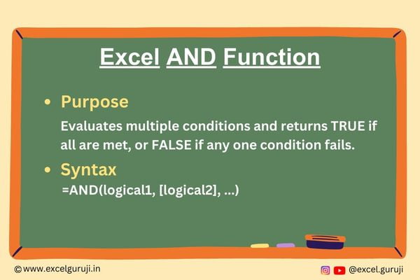
Excel AND function comes in handy when you want to evaluate two or more conditions and determine if all of them are true. It returns TRUE if all conditions are met and FALSE if any one of them is not satisfied. Here are some common situations where you might use the AND function:

Data Validation: You can use AND to validate data entries by checking multiple conditions. For example, ensuring that a value falls within a certain range and meets specific criteria simultaneously.

Conditional Formatting: Apply conditional formatting to cells based on multiple criteria. For instance, highlight cells that meet both color and value conditions.

Business Logic: In financial modeling or data analysis, you may need to check if several conditions are met before making a decision or calculation.

Inventory Management: Use the AND function to verify if the quantity and price of a product meet certain requirements before ordering more stock.

What Excel AND Function Returns

Excel AND function returns a Boolean value, which is either TRUE or FALSE. Here’s how it works:

If all the conditions specified in the AND function are TRUE, it returns TRUE.
If any of the conditions are FALSE, it returns FALSE.

Syntax of Excel AND Function

The syntax of the Excel AND function is as follows:

=AND(logical1, [logical2], …)

Input Arguments

Here are the input arguments for the Excel AND function:

● logical1, logical2, …: These are the conditions or expressions you want to evaluate. You can specify up to 255 different conditions separated by commas.

Extra Notes

● If you provide only one condition, the AND function will simply return the result of that condition.

● The conditions can be logical expressions, cell references, or values. For example, you can use A1>10 as a condition.

● You can use parentheses to group conditions and control the order of evaluation.

● Text values must be enclosed in quotation marks ” “

Examples of the Excel AND Function

Here are three examples demonstrating the usage of the AND function:

Example 1: Data Validation

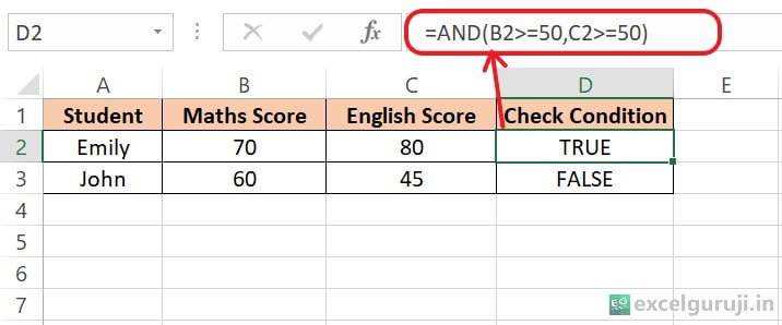
Suppose you have a list of exam scores in column B & Column C, and you want to check if a student passed both the math and English exams, with a passing score of 50 or higher. In Column D, you can use the following formula:

This formula returns TRUE only if both conditions (math score and English score) are met.

Example 2: Use With IF Function

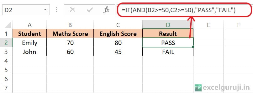
Following formula is used to determine whether a student has PASS or FAIL based on their Maths and English scores.

So, for each student, the formula checks whether both their Math and English scores are 50 or higher. If they are, it returns PASS in the Result column, indicating that the student has passed. If either of the scores is below 50, it returns FAIL, indicating that the student has failed.

Conclusion

In conclusion, the Excel AND function is a valuable tool for evaluating multiple conditions and making informed decisions in your spreadsheets. Whether you are validating data, applying conditional formatting, or implementing complex business logic, the AND function simplifies the process of ensuring all criteria are met before proceeding.

Remember, practice is key to mastering Excel functions. Experiment with different scenarios and explore the versatility of the AND function in your own projects. Start using the AND function today to enhance your Excel proficiency and streamline your data analysis tasks.

Frequently Asked Questions (FAQs)

Q1: Can the AND function be used to check if any of the conditions are true?

A1: No, the AND function specifically checks if all conditions are true. To check if any one of multiple conditions is true, you should use the Excel OR function.

Q2: Is the AND function case-sensitive when comparing text values?

A2: No, the AND function treats text values in a case-insensitive manner. “APPLE” and “apple” are considered the same.

Q3: What happens if I provide an empty cell reference as a condition in the AND function?

A3: If any condition in the AND function is an empty cell reference, it will be treated as FALSE. So, if you have conditions like =AND(A1>10, B1<=5), and B1 is empty, the result will be FALSE.

Q4: Can I use the AND function to evaluate more than 255 conditions?

A4: No, the AND function supports a maximum of 255 conditions. If you need to evaluate more conditions, you may need to use nested AND functions or find an alternative approach.

Master Date Calculations with Excel DATEDIF Function: Tips and Examples

October 4, 2023 by Excel Guruji

Excel DATEDIF Function

When to Use the Excel DATEDIF Function in Excel

Excel DATEDIF function is a powerful tool for calculating the difference between two dates in various time units such as days, months, or years. It’s particularly useful when you need to determine durations, track project timelines, or calculate ages based on birthdates.

What Excel DATEDIF Function Returns

Excel DATEDIF function returns the difference between two dates in the specified time unit, represented as a whole number. The time unit is determined by the third argument, which is user-defined.

Syntax of Excel DATEDIF Function

The syntax of the Excel DATEDIF function is as follows:

=DATEDIF(start_date, end_date, unit)

Input Arguments

Here are the input arguments for the Excel DATEDIF function:

● start_date: The starting date, which can be a reference to a cell containing a date or a direct date entry enclosed in quotation marks. It can also be a formula that evaluates to a date.

● end_date: The ending date, which can be a reference to a cell containing a date or a direct date entry enclosed in quotation marks. It can also be a formula that evaluates to a date.

● unit: The unit of time for which you want to calculate the difference. This argument should be one of the following text values:

‘Y’ (Years): Returns the count of complete years in the period between start_date and end_date.
‘M’ (Months): Returns the count of complete months in the period between start_date and end_date, regardless of the day within each month.
‘D’ (Days): Returns the count of complete days in the period between start_date and end_date, without considering months or years.
‘MD’ (Month-Day Difference): Calculates and returns the difference in days between start_date and end_date, while ignoring the months and years.
‘YM’ (Year-Month Difference): Computes and returns the difference in months between start_date and end_date, disregarding the days and years.
‘YD’ (Year-Day Difference): Computes and returns the difference in days between start_date and end_date, taking only the years into account and ignoring the months.

Extra Notes

● Excel DATEDIF function is not documented in Excel’s function wizard, but it is a valid function.

● The function does not provide fractional results; it always returns whole numbers.

● Excel DATEDIF function comes in handy in scenarios where you require age calculations.

● If the start_date is later than the end_date, the function will produce the #NUM! error as the result.

Examples of the Excel DATEDIF Function

Here are three examples demonstrating the usage of the DATEDIF function:

Example 1: Basic Usage

Suppose you have a list of birthdates in column A, and you want to calculate the age of each person as of today (current date). In column B, you can use the following formula:

This formula calculates the age in years.

Example 2: Tracking Project Duration

If you are managing a project and need to track the number of days it has been running, you can use the DATEDIF function. Let’s say the start date is in cell A2, and the end date is in cell B2. In cell C2, you can use the formula:

This formula calculates the number of days between the two dates.

Example 3: Determining Months of Employment

Suppose you have a list of employee hire dates in column A, and you want to calculate the number of months each employee has been with the company. In column B, you can use the formula:

This formula calculates the months of employment.

Conclusion

In conclusion, the Excel DATEDIF function is a valuable tool for calculating date differences in various time units. Whether you need to calculate ages, track project durations, or determine lengths of employment, the DATEDIF function can simplify your date-related calculations and enhance your Excel proficiency.

Remember, Excel offers a wide range of functions, and mastering them takes practice. Don’t hesitate to experiment and explore different applications of the DATEDIF function in your own projects. Start using the DATEDIF function today and take your Excel skills to the next level!

Frequently Asked Questions (FAQs)

Q1: Can the DATEDIF function calculate time differences in hours or minutes?

A1: No, the DATEDIF function is designed to calculate differences in days, months, or years. For more precise time calculations, you may need to use other Excel functions or formulas.

Q2: Is the DATEDIF function available in all versions of Excel?

A2: The DATEDIF function is available in most versions of Excel, including Excel 2013 and later. However, it may not be documented in the function wizard.

Q3: Are there any limitations to using the DATEDIF function?

A3: While the DATEDIF function is useful for many date calculations, it may not account for all specific requirements. Complex date calculations may require custom formulas or VBA macros.

Other Related Excel Functions

NETWORKDAYS,INTL Function

Excel Online Test 7

January 24, 2024September 30, 2023 by Excel Guruji

Taking this Excel online test is more than just showing your skills. It is a chance to grow and get better. Each question helps you learn!

When you finish the quiz, please share your thoughts, feedback, or even your score in the comments below. Your comments help us improve and understand what you need. So, give it your best try, and when you’re done, remember to leave a comment.

We really appreciate you being part of the excelguruji.in community!

Unleash your Excel potential! Click below to explore our extensive quiz library. Whether you are a novice or a seasoned pro, there is a quiz just for you.

Click Here to Explore More Quiz

Your path to Excel mastery continues. Enjoy the quizzes and keep conquering new heights!

Mastering Excel WEEKDAY Function: Day of the Week Calculation Made Easy

October 5, 2023September 29, 2023 by Excel Guruji

Excel WEEKDAY Function

When to Use the Excel WEEKDAY Function in Excel

The WEEKDAY function in Excel comes into play whenever you need to determine the day of the week for a given date. This can be useful in various scenarios, including:

Scheduling: When you want to know which day of the week a certain event falls on.

Deadline Management: When you need to calculate the days remaining until a project’s deadline.

Data Analysis: When you’re working with time-based data and want to group or categorize it by weekdays.

What Excel WEEKDAY Function Returns

The Excel WEEKDAY function returns an integer representing the day of the week for a given date. By default, it returns values ranging from 1 (Sunday) to 7 (Saturday), but you can customize this behavior using optional arguments.

Syntax of Excel WEEKDAY Function

The syntax of the Excel WEEKDAY function is as follows:

=WEEKDAY(serial_number, [return_type])

Input Arguments

Here are the input arguments for the Excel WEEKDAY function:

● serial_number: This is the date for which you want to find the day of the week. It can be a reference to a cell containing a date, a date entered directly in the formula, or a function that returns a date.

● return_type (optional): This argument allows you to specify the type of result you want:

return_type = 1 (default): Returns values from 1 (Sunday) to 7 (Saturday).
return_type = 2: Returns values from 1 (Monday) to 7 (Sunday).
return_type = 3: Returns values from 0 (Monday) to 6 (Sunday).
And more, depending on your specific needs.

Note : No need to memorize the numeric value; it will be displayed when you enter the formula.

Extra Notes

● If return_type is omitted, Excel assumes it to be 1.

● If the serial_number falls outside the current date base value range, you’ll receive a #NUM! error.

● Similarly, if the return_type is beyond the range provided in the table above, a #NUM! error will be returned.

● Excel WEEKDAY function returns a value 7 even when the referenced cell is empty.

● When using return_type 3, the WEEKDAY function returns 0 for dates that fall on a Monday.

● The WEEKDAY function can handle both date and time values, but it only evaluates the date component.

Examples of the Excel WEEKDAY Function

Here are three examples demonstrating the usage of the WEEKDAY function:

Example 1: Basic Usage

Suppose cell A2 contains the date 29-09-2023, and you want to find out which day of the week it is. In cell B2, use the following formula:

This will return 6, indicating that September 29, 2023, falls on a Friday.

Example 2: Conditional Formatting to Highlight Weekends

Imagine you have a spreadsheet with a list of dates in column A, and you want to visually identify weekends for better data analysis. In this example, we will explore more advanced applications of conditional formatting.

Let’s explain the conditional formatting process step by step.

Step 1: Select the cells on which you want to apply conditional formatting

Step 2: Go to the Home tab in the Excel ribbon. In the Styles group, you will find the Conditional Formatting button. Click on it.

Step 3: In the dropdown menu that appears when you click Conditional Formatting, choose New Rule.

Step 4: In the New Formatting Rule dialog box, select Use a formula to determine which cells to format.

Step 5: In the formula box, enter the following formula: =OR(WEEKDAY($A2) = 1, WEEKDAY($A2) = 7)

Step 6: Click the Format button next to the formula box. A Format Cells dialog box will appear.

Step 7: In the Format Cells dialog box, go to the Fill tab. Choose a background color to highlight the cell when the condition is met.

Step 8: Click OK to close the Format Cells dialog box. Back in the New Formatting Rule dialog box, Click OK to apply the formatting.

Now, all the cells that correspond to Saturday and Sunday will be highlighted.

Conclusion

In summary, the Excel WEEKDAY function is an invaluable tool for working with dates and understanding the corresponding day of the week. Whether you are planning your schedule, managing deadlines, or analyzing time-related data, the WEEKDAY function can simplify your tasks and enhance your Excel proficiency.

Remember, practice is key to mastering Excel functions, so don’t hesitate to experiment and explore different applications of the WEEKDAY function in your own projects. Start using the WEEKDAY function today and elevate your Excel skills to new heights!

Frequently Asked Questions (FAQs)

Q1: Can the WEEKDAY function return the day of the week as text?

A1: The WEEKDAY function by itself returns an integer, but you can use other Excel functions (like CHOOSE or TEXT) to convert the numeric result into text form.

Q2: Can the WEEKDAY function handle date and time values?

A2: Yes, the WEEKDAY function can handle date and time values, but it evaluates only the date component.

Q3: What does the return_type argument in WEEKDAY function do?

A3: The return_type argument allows you to customize the range of values returned by the WEEKDAY function, including options for different starting days of the week.

Q4: Can the WEEKDAY function be used to find the day of the week for dates in the past?

A4: Yes, the WEEKDAY function can handle both future and past dates, allowing you to find the day of the week for any date in history.

Other Related Excel Functions

NETWORKDAYS,INTL Function

Excel WORKDAY.INTL Function: Boost Productivity with Efficient Scheduling [2023 Guide]

September 28, 2023 by Excel Guruji

Excel WORKDAY.INTL Function

When to Use the Excel WORKDAY.INTL Function in Excel

Excel WORKDAY.INTL function is particularly useful when you need to:

Calculate Project Deadlines: You can use it to find out when a project will be completed by considering workdays and excluding non-working days, such as weekends and holidays.

Schedule Employee Shifts: If you manage employee schedules and want to determine specific workdays for shifts, this function can be a lifesaver.

Forecast Financial Transactions: When projecting future financial transactions or investment returns, you may want to skip weekends and holidays in your calculations.

Plan Deliveries and Shipments: Businesses often use this function to schedule deliveries or shipments to ensure they occur on working days.

What Excel WORKDAY.INTL Function Returns

Excel WORKDAY.INTL function returns a date that is a specified number of workdays in the future or past, based on the provided parameters. It factors in weekends and holidays, allowing you to get precise results for your business needs.

Syntax of Excel WORKDAY.INTL Function

The syntax of the Excel WORKDAY.INTL function is as follows:

=WORKDAY.INTL(start_date, days, [weekend], [holidays])

Input Arguments

Here are the input arguments for the Excel WORKDAY.INTL function:

● start_date: This is the starting date from which you want to calculate workdays.

● days: The number of workdays to add (positive value) or subtract (negative value) from the start_date.

● weekend (optional): This argument allows you to specify which days of the week are considered weekends. A weekend is a numerical or string representation used to define the occurrence of weekends.

You can use a code to represent weekend days. For example, “0000101” considers Friday and Sunday as weekends, while “1111100” considers Monday through Friday as weekends.

You can also use numeric value for this like 2 number will represent Sunday and Monday as weekend, while 3 number will represent Monday and Tuesday as weekend. You don’t need to remember the numeric value, it will be shown to you when you enter the formula

● holidays (optional): An optional range of dates representing holidays that you want to exclude from your workday calculations.

Extra Notes

● If you omit the weekend and holidays arguments, Excel WORKDAY.INTL function assumes standard weekends (Saturday and Sunday) and no holidays.

● The WORKDAY.INTL function is a versatile tool that can handle both positive and negative values for the days argument. Positive values project future dates, while negative values calculate past dates.

● When any of the arguments isn’t a valid date, WORKDAY.INTL will result in an #VALUE! error.

● The holidays argument is also optional. If you don’t have any holidays to consider, you can omit it.

Examples of the Excel WORKDAY.INTL Function

Here are a few examples of how to use the WORKDAY.INTL function:

Example 1: Basic Usage

Suppose you want to calculate the date, considering Saturday and Sunday as weekends. Use the following formula:

=WORKDAY.INTL(A2, B2): In this example, the default WORKDAY.INTL function is used, which considers Saturday and Sunday as weekends by default. So, it calculates the date from October 1, 2023, and correctly returns the date 27-10-2023, excluding weekends.

=WORKDAY.INTL(A3, B3, “0000011”): Here, the formula includes the weekend argument “0000011” which specifies that only Saturday and Sunday are considered weekends. This configuration is the same as the default, so it also the date from October 1, 2023, and correctly returns date 27-10-2023.

=WORKDAY.INTL(A4, B4, 1): In this case, the weekend argument is specified as the number 1, which also specifies that only Saturday and Sunday are considered weekends.

Example 2: Custom Weekend Days

Let’s say your organization follows a different workweek, with only Tuesday as weekends. So, you can calculate working days using the following formulas:

=WORKDAY.INTL(A2, B2, “0100000”): Here, the formula includes the weekend argument “0100000” which specifies that only Tuesday is considered weekends.

=WORKDAY.INTL(A3, B3, 13): In this case, the weekend argument is specified as the number 13, which also specifies that only Tuesday is considered weekends.

Example 3: Including Holidays

If you have specific holidays to account for, let’s say, in cells A5:A6, you have a list of holiday dates, and you want to calculate the date, while also considering Tuesday and Friday as weekends, you can use the following formula:

Conclusion

In conclusion, the Excel WORKDAY.INTL function is an indispensable tool for calculating workdays accurately while considering custom weekend settings and holidays.

Whether you’re managing projects, schedules, or financial forecasts, this function can help you make informed decisions and meet your deadlines with ease.

Don’t hesitate to experiment with different scenarios and adapt the WORKDAY.INTL function to your specific needs. Excel’s flexibility allows you to tackle a wide range of real-world challenges effectively.

Frequently Asked Questions (FAQs)

Q1: Can the WORKDAY.INTL function calculate workdays based on non-standard weekends?

A1: Yes, you can customize the weekend parameter in the WORKDAY.INTL function to define non-standard weekends. This allows you to adapt the function to different workweek schedules.

Q2: Can I use the WORKDAY.INTL function to calculate workdays within a range of dates?

A2: No, the WORKDAY.INTL function calculates workdays based on a starting date and the number of workdays to add or subtract. To calculate workdays within a date range, you may need to use other functions in combination with WORKDAY.INTL.

Q3: What happens if the number of workdays specified in the WORKDAY.INTL function exceeds the date range in the future or past?

A3: If the number of workdays exceeds the available workdays in the specified direction (future or past), the function will return a date beyond the date range. You may need to adjust the start date or the number of workdays to stay within the desired range.

Q4: Can I use the WORKDAY.INTL function to calculate workdays for multiple rows or cells at once?

A4: Yes, you can apply the WORKDAY.INTL function to a range of cells by entering it as an array formula or by dragging it across multiple cells. Just make sure the input arguments are correctly adjusted for each cell in the range.

Other Related Excel Functions

NETWORKDAYS,INTL Function

Mastering Excel WORKDAY Function: Efficient Date Calculations

September 28, 2023September 28, 2023 by Excel Guruji

Excel WORKDAY Function

When to Use the Excel WORKDAY Function in Excel

Excel WORKDAY function is used in scenarios where you want to calculate a date that falls a certain number of workdays ahead or behind a given date. This function is commonly employed in business and project management to schedule tasks, estimate delivery dates, and manage project timelines.

What Excel WORKDAY Function Returns

Excel WORKDAY function returns a date that is a specified number of workdays (business days) ahead or behind a given start date. It allows you to skip weekends (Saturdays and Sundays) and optionally, any specified holidays, making it a valuable tool for accurate date calculations.

Syntax of Excel WORKDAY Function

The syntax of the Excel WORKDAY function is as follows:

=WORKDAY(start_date, days, [holidays])

Input Arguments

Here are the input arguments for the Excel WORKDAY function:

● start_date: This is the initial date from which you want to calculate the workdays. It can be a reference to a cell containing a date or a direct date entry enclosed in quotation marks.

● days: The number of workdays (positive or negative) you want to add or subtract from the start_date. This argument can also be a cell reference containing the number of days.

● holidays (optional): This argument is not mandatory. You can provide a list of dates (range or array) that represent holidays when work should not be considered. If omitted, weekends (Saturdays and Sundays) are the only days excluded.

Extra Notes

● If you use a negative value for the days argument, the WORKDAY function will calculate dates in the past from the start_date.

● If your holiday list is subject to change, consider storing it in a separate range or table in your Excel workbook and referencing that range in your WORKDAY function. This way, you can easily update the list without modifying your formulas.

● If any of the arguments is not a valid date, the WORKDAY function will result in an error, displaying #VALUE!.

● Additionally, if the addition of start_date and days results in an invalid date, WORKDAY will return the #NUM! error value.

● It is worth noting that if the days argument is not an integer, Excel will truncate it.

Examples of the Excel WORKDAY Function

Here are a few examples of how to use the WORKDAY function:

Example 1: Calculating a Future Date

Suppose you have a project that starts on October 1, 2023, and you want to know the date 15 workdays into the project. You can use the following formula:

This formula will return the serial number of a date. If you want to convert it into a date format, go to the Home tab, and then select Short Date or Long Date from the Number Format ribbon.

Example 2: Accounting for Holidays

In a business scenario where holidays are observed, you can include a list of holidays to ensure accurate calculations. For example:

This formula calculates a date twenty workdays from October 1, 2023, excluding all weekends and holidays.

Conclusion

In conclusion, the Excel WORKDAY function is an essential tool for handling date calculations in a business context. Whether you need to plan project timelines, estimate delivery dates, or manage work schedules, this function simplifies the process by excluding non-working days.

By mastering the Excel WORKDAY function, you can enhance your efficiency in Excel and improve your ability to manage time-sensitive tasks accurately.

Remember, Excel offers a wide range of date and time functions, so exploring and experimenting with them can lead to more efficient data management and analysis in your projects. Start using the Excel WORKDAY function today and take your Excel skills to the next level!

Frequently Asked Questions (FAQs)

Q1: Can the WORKDAY function handle negative values to calculate past dates?

A1: Yes, the WORKDAY function can handle negative values to calculate dates in the past by subtracting workdays from the start_date.

Q2: Can I use cell references for the start_date and days arguments?

A2: Absolutely, you can use cell references for both the start_date and days arguments, which makes your formulas dynamic and easily updatable.

Q3: Is it necessary to provide holidays as an argument in the WORKDAY function?

A3: No, it is not mandatory to provide holidays. If omitted, the function will only exclude weekends (Saturdays and Sundays) from the calculation.

Q4: Can the WORKDAY function handle regional date formats?

A4: Yes, the WORKDAY function is flexible and can handle various date formats based on your system settings, making it suitable for international users.

Q5: How do I calculate workdays excluding only specific weekdays, not weekends?

A5: If you want to exclude specific weekdays (e.g., Mondays and Wednesdays), you can use a Excel WORKDAY.INTL functions to achieve this custom calculation.

Other Related Excel Functions

DAY Function

DATE Function

NETWORKDAYS Function

NETWORKDAYS.INTL Function

Mastering Excel NETWORKDAYS.INTL Function: Calculate Workdays with Precision!

September 28, 2023September 27, 2023 by Excel Guruji

Excel NETWORKDAYS.INTL Function

When to Use the Excel NETWORKDAYS.INTL Function in Excel

Excel NETWORKDAYS.INTL function is a powerful tool for calculating the number of working days between two dates while allowing you to customize which days of the week are considered non-working days. It is particularly useful for businesses and organizations that have non-standard workweeks or holidays that fall on different days.

What Excel NETWORKDAYS.INTL Function Returns

The Excel NETWORKDAYS.INTL function returns the count of working days between two specified dates, considering your defined weekend days and any specified holidays.

Syntax of Excel NETWORKDAYS.INTL Function

The syntax of the Excel NETWORKDAYS.INTL function is as follows:

=NETWORKDAYS.INTL(start_date, end_date, [weekend], [holidays])

Input Arguments

Here are the input arguments for the Excel NETWORKDAYS.INTL function:

● start_date: This is the start date of the period for which you want to calculate working days.

● end_date: This is the end date of the period for which you want to calculate working days.

Excel-NETWORKDAYS.INTL-Function-Argument

● holidays (optional): You can provide a range of dates that represent holidays. These dates will be excluded from the calculation.

Extra Notes

● If you omit the weekend argument, it defaults to considering only Saturday and Sunday as weekends.

● The start_date and end_date arguments should be valid date values.

● If the start_date is after the end_date, the result will be a negative value, indicating the total count of complete workdays between them.

● When any of the arguments isn’t a valid date, NETWORKDAYS.INTL will result in an #VALUE! error.

● The holidays argument is also optional. If you don’t have any holidays to consider, you can omit it.

Examples of the Excel NETWORKDAYS.INTL Function

Here are a few examples of how to use the NETWORKDAYS.INTL function:

Example 1: Basic Usage

Suppose you want to calculate the number of working days between two dates, considering Saturday and Sunday as weekends. Use the following formula:

Excel NETWORKDAYS.INTL Function Example 1 1

=NETWORKDAYS.INTL(A2, B2): In this example, the default NETWORKDAYS.INTL function is used, which considers Saturday and Sunday as weekends by default. So, it calculates the number of working days between September 1, 2023, and September 20, 2023, and correctly returns 14, excluding weekends.

=NETWORKDAYS.INTL(A3, B3, “0000011”): Here, the formula includes the weekend argument “0000011” which specifies that only Saturday and Sunday are considered weekends. This configuration is the same as the default, so it also calculates 14 working days, excluding the weekends.

=NETWORKDAYS.INTL(A4, B4, 1): In this case, the weekend argument is specified as the number 1, which also specifies that only Saturday and Sunday are considered weekends.

Example 2: Custom Weekend Days

Let’s say your organization follows a different workweek, with only Sunday as weekends. So, you can calculate working days using the following formulas:

=NETWORKDAYS.INTL(A2, B2, “0000001”): Here, the formula includes the weekend argument “0000001” which specifies that only Sunday is considered weekends.

=NETWORKDAYS.INTL(A3, B3, 11): In this case, the weekend argument is specified as the number 11, which also specifies that only Sunday is considered weekends.

Example 3: Including Holidays

If you have specific holidays to account for, let’s say, in cells A5:A6, you have a list of holiday dates, and you want to calculate working days between two dates while also considering Monday and Sunday as weekends, you can use the following formula:

Conclusion

In summary, the Excel NETWORKDAYS.INTL function is a versatile tool for calculating working days between two dates while accommodating custom workweeks and holidays. It’s especially valuable for businesses and organizations with unique work schedules.

By mastering the NETWORKDAYS.INTL function, you can streamline your date-related calculations and ensure accurate tracking of working days, helping you plan projects, manage resources, and meet deadlines effectively.

Frequently Asked Questions (FAQs)

Q1: Can the NETWORKDAYS.INTL function handle non-consecutive weekends, such as Thursday and Sunday?

A1: Yes, you can specify any combination of days as weekends using the weekend argument, allowing for flexible customization.

Q2: What happens if the start_date is after the end_date?

A2: If the start_date is later than the end_date, the function will return a negative number.

Q3: Can I use the NETWORKDAYS.INTL function to calculate working hours instead of days?

A3: No, the NETWORKDAYS.INTL function calculates the number of whole working days between two dates, not working hours.

Q4: Is it possible to use cell references for the weekend and holidays arguments?

A4: Yes, you can reference cells that contain the weekend and holidays codes or ranges. This allows for dynamic customization of the function.

Q5: What if I want to calculate working days without excluding any holidays?

A5: If you don’t have holidays to exclude, you can omit the holidays argument, and the function will only consider weekends.

Other Related Excel Functions

DAY Function

DATE Function

NETWORKDAYS Function

Excel NETWORKDAYS Function: Effortless Working Day Calculations

September 27, 2023September 27, 2023 by Excel Guruji

Excel NETWORKDAYS Function

When to Use the Excel NETWORKDAYS Function in Excel

Excel NETWORKDAYS function is a valuable tool when you need to calculate the number of working days between two dates. It is particularly useful in scenarios where you want to determine deadlines, project durations, or simply track the number of business days between two events.

What Excel NETWORKDAYS Function Returns

The Excel NETWORKDAYS function returns the count of working days (weekdays) between two specified dates. It excludes weekends and allows for the consideration of custom holidays, making it a versatile function for various business and project management tasks.

Syntax of Excel NETWORKDAYS Function

The syntax of the Excel NETWORKDAYS function is as follows:

=NETWORKDAYS(start_date, end_date, [holidays])

Input Arguments

Here are the input arguments for the Excel NETWORKDAYS function:

● start_date: This is the beginning date from which you want to start counting working days. It can be a reference to a cell containing a date, a direct date entry enclosed in quotation marks, or a formula that evaluates to a date.

● end_date: This is the end date up to which you want to count working days. Similar to start_date, it can be a cell reference, a direct date entry, or a formula result.

● holidays (optional): This argument allows you to specify a range of cells containing holiday dates to be excluded from the calculation. Holidays are optional, and you can omit this argument if you don’t need to consider holidays.

Extra Notes

● The NETWORKDAYS function considers Monday through Friday as working days and excludes weekends (Saturday and Sunday) by default.

● If you provide a range of holiday dates in the holidays argument, these dates will also be excluded from the count.

● When any of the arguments isn’t a valid date, NETWORKDAYS will result in an #VALUE! error.

Examples of the Excel NETWORKDAYS Function

Here are a few examples of how to use the TODAY function:

Example 1: Basic Usage

Suppose you have a project that starts on September 1, 2023 (cell A3) and ends on September 20, 2023 (cell B3). To calculate the number of working days for this project, you can use the following formula:

This formula will return the result of 14, as there are 14 working days between these two dates, excluding weekends (Saturday, Sunday).

Example 2: Including Holidays

In a project that spans multiple weeks, you may want to account for holidays. Suppose you have a list of holidays in cells A6 to A7. You can modify the formula as follows:

Now, the function will also exclude the holidays specified in the range A6:A7 from the calculation.

Example 3: Nested Functions with IF and TODAY()

You want to display a message based on the number of working days remaining until a project deadline. If the deadline is more than the working days away, display Plenty of time, otherwise, display Hurry up!

=IF(NETWORKDAYS(A3, TODAY()) < B3, “Plenty of time”, “Hurry up!”): This formula calculates the number of working days between the project start date (A3) and the current date (TODAY()) using the NETWORKDAYS function. Then, it compares this calculated value to the number of working days required to complete the project (B3).

If the calculated number of working days is less than the days required to complete the project, it means there is Plenty of time.
If the calculated number of working days is equal to or greater than the days required to complete the project, it means you need to Hurry up!.

Conclusion

In summary, the Excel NETWORKDAYS function is an essential tool for anyone working with date-related calculations in a business context.

It simplifies the process of counting working days and allows for the exclusion of weekends and holidays, making it ideal for project management, scheduling, and deadline tracking.

As you become more proficient in Excel, you will find that mastering functions like NETWORKDAYS can significantly improve your productivity and accuracy in handling date-related tasks. So, start using NETWORKDAYS today, and unlock its potential for your Excel projects!

Frequently Asked Questions (FAQs)

Q1: Can the NETWORKDAYS function be used to calculate the number of days, including weekends?

A1: No, the NETWORKDAYS function is specifically designed to calculate the number of working days, excluding weekends.

Q2: Can I use NETWORKDAYS to calculate working days for irregular workweeks (e.g., Monday, Wednesday, Friday only)?

A2: No, The NETWORKDAYS function in Excel does not directly support irregular workweeks; it is designed for standard Monday-through-Friday workweeks. Additionally, it may exclude holidays in calculation. If you want to calculate working days for irregular workweeks you can use NETWORKDAYS.INTL function

Q3: Is it possible to use NETWORKDAYS to calculate partial days (e.g., half a working day)?

A3: No, NETWORKDAYS counts whole working days. If you need to calculate partial days, you may need to use a different approach or formula.

Other Related Excel Functions

DAY Function

DATE Function