Contents
Excel AVERAGEIF Function
When to Use the Excel AVERAGEIF Function in Excel
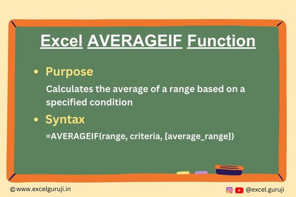
The AVERAGEIF function in Excel comes in handy when you need to calculate the average of a range based on a specific condition. This powerful function allows you to filter data and perform average calculations only for the cells that meet a specified criterion.
What Excel AVERAGEIF Function Returns
The Excel AVERAGEIF function returns the average of a range that meets a given condition.
Syntax of Excel AVERAGEIF Function
The syntax of the Excel AVERAGEIF function is as follows:
=AVERAGEIF(range, criteria, [average_range])
Input Arguments
Here are the input arguments for the Excel AVERAGEIF function:
● range: The range of cells that you want to apply the criteria to. It can be a single column or row, or a combination of both.
● criteria: The condition that determines which cells to average. This can be expressed as a number, expression, cell reference, or text string.
● [average_range]: (Optional) The actual cells to average. If this argument is omitted, the cells in the provided range are used for the calculation.
Examples of the Excel AVERAGEIF Function
Here are few examples demonstrating the usage of the AVERAGEIF function in Excel:
Example 1: Basic Usage
Suppose you have a range of sales quantities in column B, and you want to find the average for those items whose sales are above or equal to 90. In cell D2, use the following formula:
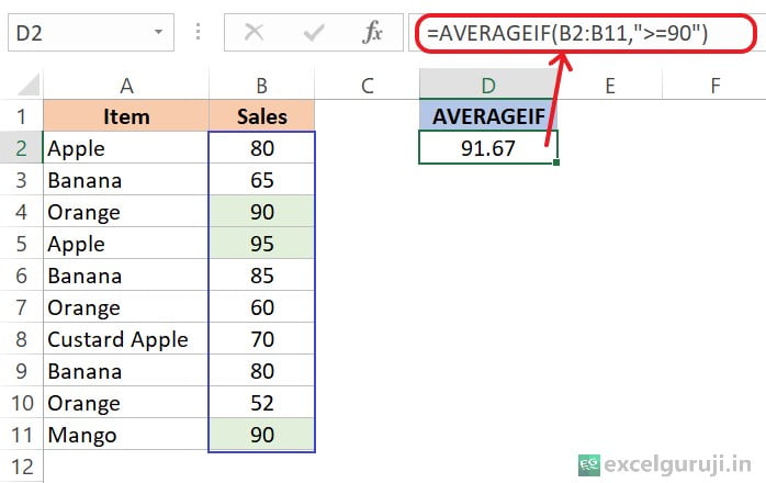
In the above example, in the second argument ‘criteria’, we used the greater than or equal to (“>=90”) operator. Consequently, the average of the cells that are greater than 90 or equal to 90 from the range will be the output.
Note: Here, we omitted the third argument [average_range], so the calculation uses the cells in the provided range.
Example 2: Averaging a Specific Range
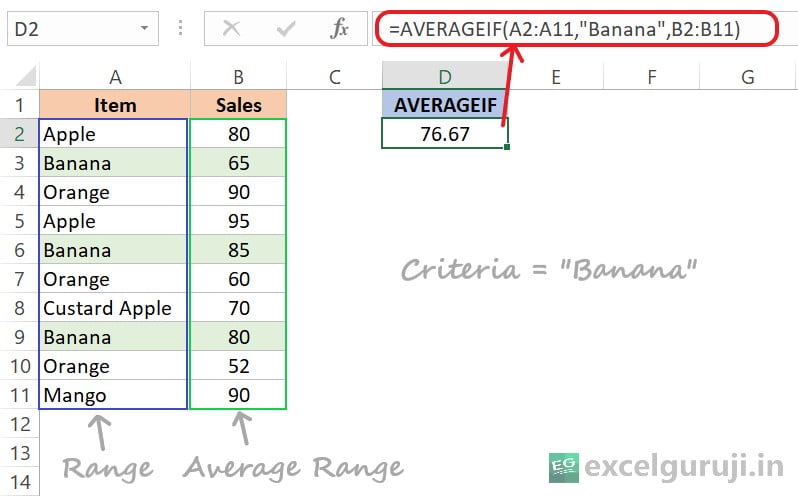
Now, suppose we have fruit items in column A and corresponding sales quantity in column B, and we want to find the average quantity for the item ‘Banana’. Use the formula:
Example 3: Using Criteria from a Cell
We will consider the above dataset in this example. We will explore a scenario where you don’t have to type the criteria every time; instead, you can use a cell reference.
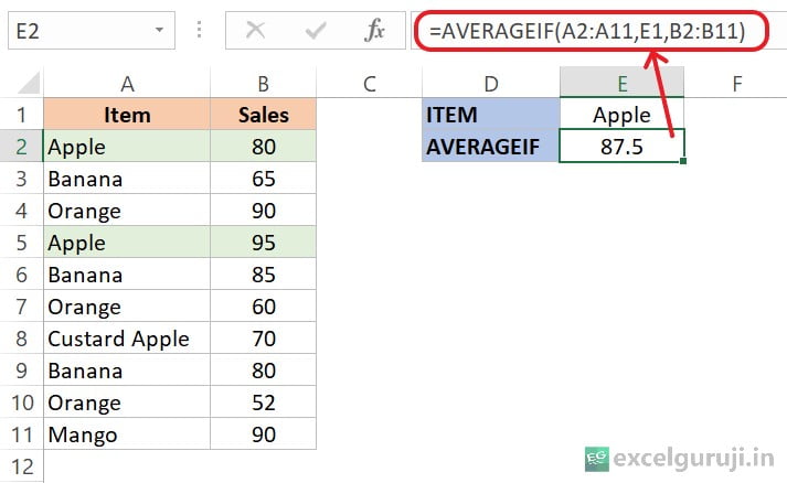
In the example above, we didn’t do anything different. But instead of typing in the criteria each time, we used a cell reference (E1).
This is helpful because you don’t have to keep changing the formula. Just update the content in the referenced cell, and the formula will automatically adjust.
Example 4: Find the Average Using Wildcard Characters
Imagine you have a sales dataset for various fruits. Now, you want to find the average sales quantity not only for ‘Apple’ but for any item that includes the term ‘Apple’ in its name. Let’s explore how you can achieve this using the AVERAGEIF function with wildcard characters.
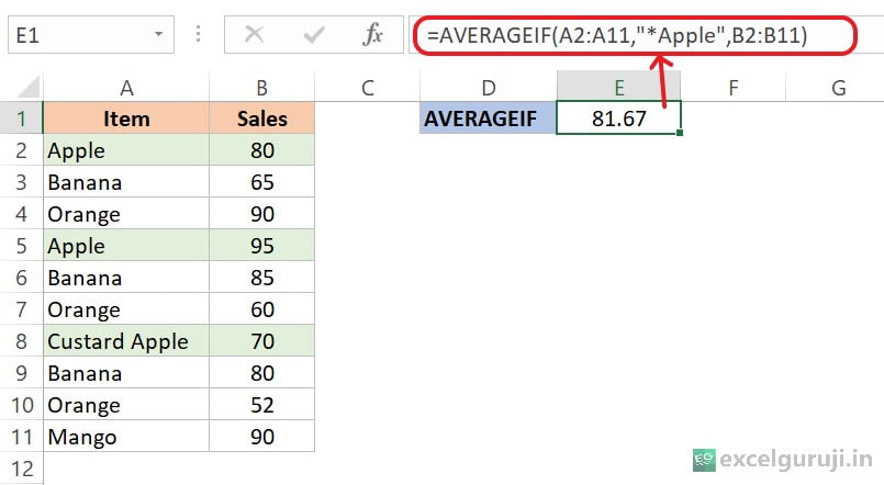
The formula =AVERAGEIF(A2:A11, “Apple”, B2:B11) calculates the average sales quantity for items containing the word “Apple” in the given data, using the wildcard (*) to match variations like “Apple” and “Custard Apple”.
Example 5: Find the Average Excluding Zero
Imagine you have a list of sales quantities for various products. Some entries contain zeros, representing instances where no sales occurred.
Now, you want to find the average sales quantity, excluding any instances where sales were zero. Let’s explore how you can achieve this using the AVERAGEIF function in Excel.
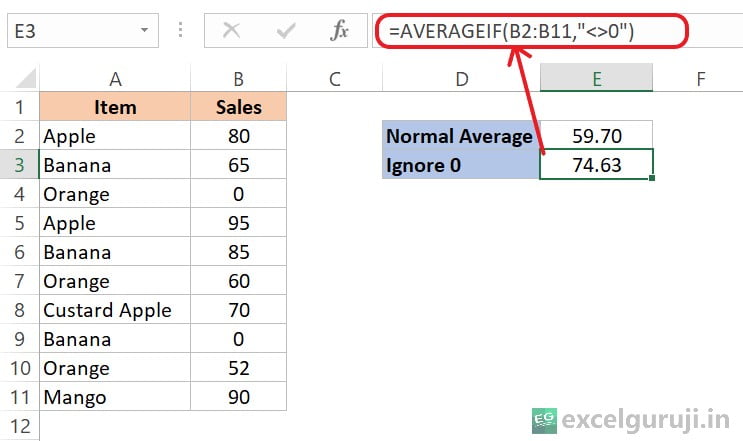
The formula =AVERAGEIF(B2:B11, “<>0”) calculates the average of numbers in the range B2:B11, excluding cells with the value 0.
Extra Notes
● If you don’t have valid numbers in what you are calculating, you will get an error: #DIV/0!
● If the provided criteria is empty, AVERAGEIF interprets it as a value of 0.
● Incorporating wildcard characters like the asterisk (*) or tilde (~) in the criteria significantly improves the search capabilities of the function. Example 4 demonstrates an effective use of wildcard characters.
● TRUE and FALSE values are disregarded when calculating an average.
● Empty cells are excluded from the average calculation.
● Excel AVERAGEIF function accommodates wildcards but operates in a case-insensitive manner.
Practice Workbook
There are two sheets in the practice file
Download Free Excel File For PracticeConclusion
In conclusion, the Excel AVERAGEIF function is a versatile tool for calculating averages based on specific conditions. Whether you are analyzing performance data, survey results, or any numeric values, the AVERAGEIF function allows you to tailor your calculations to meet your exact needs.
As you explore and apply the AVERAGEIF function in your Excel projects, you will discover its effectiveness in streamlining data analysis and gaining valuable insights. Don’t hesitate to experiment with different criteria and scenarios to enhance your proficiency in using the AVERAGEIF function.
Frequently Asked Questions (FAQs)
Q1: Can the AVERAGEIF function be used with text criteria?
A1: Yes, the AVERAGEIF function supports text criteria, allowing you to filter and calculate averages based on specific text conditions.
Q2: Is it possible to use multiple criteria with the AVERAGEIF function?
A2: For multiple criteria, you should use the AVERAGEIFS function, which extends the capabilities of AVERAGEIF to handle multiple conditions.
Q3: What happens if the specified range or criteria are empty?
A3: If the range or criteria is empty, the AVERAGEIF function returns an error.
Q4: Can the AVERAGEIF function be used with dates?
A4: Yes, the AVERAGEIF function can be used with date criteria to calculate averages based on specific date conditions.
Other Related Excel Functions
Mastering Excel AVERAGEIFS Function: A Comprehensive Guide to Conditional Averaging in Data Analysis
Excel AVERAGE Function: Elevate Your Data Analysis Game
Unlocking the Power of Excel COUNT Function for Accurate Numeric Data Analysis
Join me on Instagram, YouTube and WhatApp Channel for your daily dose of valuable tips and tricks! Catch insightful videos that will enhance your knowledge and skills. Don’t miss out – follow me now!