Contents
- 1 Excel HLOOKUP Function
- 2 When to Use the Excel HLOOKUP Function in Excel
- 3 What Excel HLOOKUP Function Returns
- 4 Syntax of Excel HLOOKUP Function
- 5 Input Arguments
- 6 Extra Notes
- 7 Examples of the Excel HLOOKUP Function
- 8 Practice with Real Examples: Download the Attached Excel File
- 9 Conclusion
- 10 Frequently Asked Questions (FAQs)
Excel HLOOKUP Function

When to Use the Excel HLOOKUP Function in Excel
The HLOOKUP function in Excel is a powerful tool when you need to search for a value in the first row of a range and retrieve a corresponding value in the same column from a specified row. This function is particularly useful when dealing with large datasets, tables, or spreadsheets with headers and data organized horizontally.
What Excel HLOOKUP Function Returns
The Excel HLOOKUP function returns a value by searching for a specified lookup value in the first row of a table or range and then retrieving the corresponding value from a specified row. It essentially performs a horizontal lookup in a table.
Syntax of Excel HLOOKUP Function
The syntax of the Excel HLOOKUP function is as follows
=HLOOKUP(lookup_value, table_array, row_index_num, [range_lookup])
Input Arguments
Here are the input arguments for the Excel HLOOKUP function:
● lookup_value: The value to search for in the first row of the table.
● table_array: The range of cells that contains the data. The first row of this range should contain the values to be searched.
● row_index_num: The row number in the table from which to retrieve the value.
● range_lookup [optional]: A logical value that specifies whether to find an exact match or an approximate match. If TRUE or omitted, it searches for an approximate match. If FALSE, it searches for an exact match.
Extra Notes
● If no match is found, the function returns #N/A.
● The table_array must be arranged in a way that the first row contains the values to be searched, and the subsequent rows contain the corresponding data.
● The row_index_num must be a positive integer.
● If range_lookup is TRUE or omitted, the values in the first row of table_array must be sorted in ascending order.
● Excel HLOOKUP function is case-insensitive, treating uppercase and lowercase characters as the same.
Examples of the Excel HLOOKUP Function
Here are few examples of using the HLOOKUP function in Excel
Example 1: Basic Usage
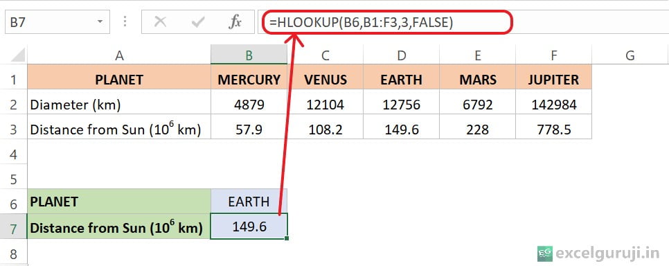
Imagine you are an astronomer working with a dataset that contains information about various planets, including their diameters and distances from the Sun1. Your goal is to use the HLOOKUP function in Excel to quickly retrieve specific details about a particular planet based on input.

Here is an explanation of the formula: =HLOOKUP(B6, B1:F3, 3, FALSE)
- B6: This is the lookup value. In this case, you are looking for the value in cell B6, which is likely a planet name (e.g., “EARTH”).
- B1:F3: This is the table array. It represents the range of cells that contains the data. In this context, it is likely the dataset with information about planets, their diameters, and distances from the Sun.
- 3: This is the row index number. It indicates from which row in the table array the function should retrieve the corresponding value. In this case, you specified 3, so it will look in the third row of the table array.
- FALSE: This is the range_lookup parameter. When set to FALSE, it indicates that an exact match is required. In other words, the function will look for the exact value specified in B6 in the first row of the table array.
Example 2: Approximate Match With HLOOKUP
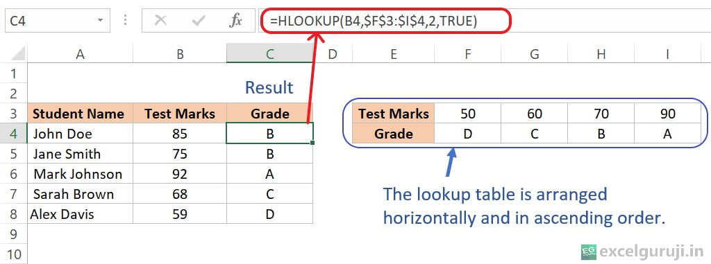
Suppose you are a teacher managing a class of students, and you want to automatically assign grades based on their test marks. You have a list of students with their respective test marks, and you have established a grading scale with specific grade ranges. To streamline the grading process, you decide to use a lookup array to automatically determine the grade for each student.

Here is an explanation of the formula: =HLOOKUP(B4,$F$3:$I$4,2,TRUE)
- B4 is the cell containing the test marks for a specific student.
- $F$3:$I$4 is the lookup array, where the dollar signs ($) make the reference absolute.
- 2 is the row index number, indicating that the function should return the corresponding grade from the second row of the lookup array.
- TRUE means it will perform an approximate match, finding the closest (lesser) value in the first row of the lookup array.
Example 3: Exact Match With HLOOKUP
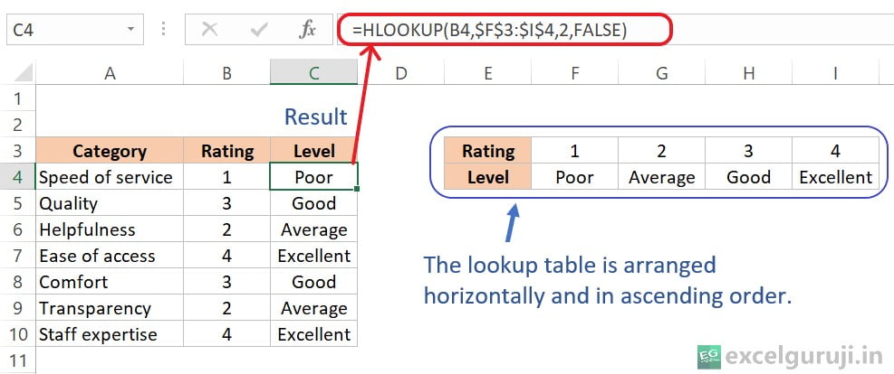
Imagine you work for a company that provides services to customers, and you have conducted a customer satisfaction survey to gather feedback on various aspects of your service. You asked customers to rate different service attributes on a scale from 1 to 4, where 1 is “Poor”, 2 is “Average”, 3 is “Good” and 4 is “Excellent”. The survey covered categories like speed of service, quality, helpfulness, ease of access, comfort, transparency, and staff expertise.

Here is an explanation of the formula: =HLOOKUP(B4, $F$3:$I$4, 2, FALSE)
- B4: This is the cell reference containing the “Rating” in data table.
- $F$3:$I$4: This is the lookup array or table. It is a where the first row contains the ratings (1, 2, 3, 4), and the second row contains the corresponding levels (Poor, Average, Good, Excellent). The $ symbols before the column and row references make the range absolute, meaning it won’t change when you copy the formula to other cells.
- 2: This parameter indicates that the function should return the value from the second row of the lookup table (which contains the levels).
- FALSE: This is the range_lookup parameter, and setting it to FALSE means that the function should find an exact match for the rating. If an exact match is not found, it returns an error (#N/A).
Practice with Real Examples: Download the Attached Excel File
To facilitate your hands-on practice, I have attached an Excel file. You can download the file and work through the three examples I shared earlier, applying the HLOOKUP function in Excel.
Download Excel FileIf you have any questions or need assistance, feel free to reach out. Enjoy practicing and mastering the Excel HLOOKUP function!
Conclusion
In conclusion, the Excel HLOOKUP function is a valuable tool for searching and retrieving data from horizontally organized tables. Whether you are working with sales data, project timelines, or any dataset where information is arranged horizontally, the Excel HLOOKUP function can streamline your data retrieval tasks.
As with any Excel function, practice is key to mastering the HLOOKUP function. Experiment with different scenarios and datasets to enhance your proficiency. Start incorporating the HLOOKUP function into your Excel repertoire today and take your data analysis skills to the next level!
Frequently Asked Questions (FAQs)
Q1: Can the Excel HLOOKUP function be used to search for values in the first column of a table?
A1: No, the Excel HLOOKUP function is designed exclusively for searching in the first row of a table.
Q2: Is the HLOOKUP function case-sensitive?
A2: No, the HLOOKUP function is not case-sensitive.
Q3: What happens if no match is found using HLOOKUP?
A3: If no match is found, the function returns #N/A.
Q4: Can the row_index_num be a negative number?
A4: No, the row_index_num must be a positive integer.
Q5: How does the HLOOKUP function handle duplicates in the first row of the table?
A5: The HLOOKUP function returns the first matching value found in the first row of the table, even if there are duplicates.
Other Related Excel Functions
Mastering Excel VLOOKUP Function: A Comprehensive Guide to Enhance Your Data Analysis Skills
Mastering Excel FILTER Function: A Comprehensive Guide for Data Filtering
Master Data Selection with Excel TAKE Function
Excel DROP Function: A Comprehensive Guide to Unlocking Excel’s Potential:
Join me on Instagram, YouTube and WhatApp Channel for your daily dose of valuable tips and tricks! Catch insightful videos that will enhance your knowledge and skills. Don’t miss out – follow me now!